Example using simulated data from a species distribution model • robust.prioritizr

Systematic conservation planning problems often involve finding least-cost solutions to ensure the representation of different species under climate change. These involve the use of future climate projection and the use of species distribution models that carry uncertainty from the use of scenarios and the model fitting process. If these uncertainties are ignored, the solution of the systematic conservation planning problems may fail to meet its targets.

In this example we walk through how someone with a climate-sensitive species distribution model can harness the flexible interface of Robust Prioritizr to identify a conservation plan that is robust to uncertainties emanating from both climate scenarios and the data modelling process.

Robust Prioritizr is agnostic to the data generating process - users who only wish to apply it to their own model can go directly to the “Model Specification” section. Some familiarity with the Prioritizr framework for solving conservation planning problems is helpful but not necessary in understanding the vignette.

Data generating process

Suppose the analyst fitted the following statistical model of the species abundance based on data: r_{ij} \sim \text{Poisson}(\theta_{ij})

\theta_{ij} = \log(\beta_0 + \beta_1 Temp_i + \beta_2 Temp_i^2 + \beta_3 Prec_i + \beta_4 Prec_i^2 + \varepsilon_{ij})

where the abundance r of species j in location i follows a Poisson distribution with the mean \theta, which is function of the climate covariates Temperature Temp and Precipitation Prec and a random i.i.d. error term \varepsilon. The relationships between the climate variables and the mean are modelled using the regression coefficients \beta_1, \beta_2, \beta_3, \beta_4. For simplicity, we assume here that its abundance only depends on these two climatic variables.

We simulate the abundance data for two species as follows:

Species 1: a species with a narrow climatic niche, best adapted to habitats with 18.5 Celsius and 1000mm of annual precipitation. Its expected abundance drops significantly once the climate move away from 17.5C and 1000mm of annual precipitation.
Species 2: a species with a wider climatic niche, best adapted to habitats with 20 Celsius and 1000mm of annual precipitation. Because it has a wider climatic niche, its abundances are still high when temperature and precipitation exceeds these optimal values.

Here, we generate the temperature and precipitation values of a simulated landscape and plot the expected abundance with respect to temperature (holding precipitation constant). As we can see in the figure below, Species 1 have a lower expected abundance, and its expected abundance declines rapidly once temperature changes away from its optimal temperature.

set.seed(19895894)
N <- 10

# Prepare baseline temperature and precipitation simulated data
m <- expand.grid(prec = seq(900, 1200, length.out = N),
                 temp = seq(16, 20, length.out = N))

temp <- matrix(m$temp + rnorm(N^2, 0, 0.2), N, N, byrow = TRUE)
prec <- matrix(m$prec + rnorm(N^2, 0, 20), N, N, byrow = TRUE)

# Find the coefficients of the model given the optimal temp/ prec and shape of the quadratic function
beta_coefs <- function(T_opt, P_opt, k_T, k_P, peak = 10) {
  beta_0 <- log(peak) + T_opt^2 * k_T/2 + P_opt^2 * k_P/2
  beta_1 <- -k_T * T_opt
  beta_2 <- k_T/2
  beta_3 <- -k_P * P_opt
  beta_4 <- k_P / 2
  return(cbind(beta_0, beta_1, beta_2, beta_3, beta_4))
}

# Specify climate abundance response function of the species, assume that its probability of occurrence
# follow a multivariate Gaussian distribution of temperature and precipitation
ab_function <- function(temp, prec, betas, sigma = 0, return_vec = F) {
  t <- as.vector(temp)
  p <- as.vector(prec)
  model_matrix <- cbind(1, t, t^2, p, p^2)
  betas <- as.vector(betas)

  v <- exp(model_matrix %*% betas + rnorm(length(t))*sigma)
  if (return_vec) return(as.vector(v))
  return(matrix(v, nrow = nrow(temp), ncol = ncol(temp)))
}

# Define function for drawing random abundance numbers based on expected abundance numbers
rpois_matrix <- function(exp_ab) {
  dim <- dim(exp_ab)
  rpois(dim[1]*dim[2], as.vector(exp_ab)) %>%
    matrix(nrow = dim[1], ncol = dim[2])
}

# Define a function that can draw abundance values based on temperature, precipitation and a matrix of beta
ab_draw_pois <- function(t, p, beta) {
  beta_rand <- as.vector(beta[sample(1:nrow(beta), 1),])
  exp_ab <- function(t, p,...) ab_function(t, p, beta_rand,...)
  rpois_matrix(exp_ab(temp, prec))
}


beta_species_1 <- beta_coefs(18.5, 1000, -.3, -.005, 10)
beta_species_2 <- beta_coefs(20, 1000, -.1, -.0001, 8)

# Define functions for species 1 and 2, controlling mu for their optimal temperature and precipitation,
# and sigma for the range it can survive in, Ntrials for scaling the absolute number of occurrences
exp_ab_1 <- function(t, p,...) ab_function(t, p, beta_species_1,...)
exp_ab_2 <- function(t, p, ...) ab_function(t, p, beta_species_2,...)

# Uncertainty in the beta parameters - suppose we estimate a model and get confidence intervals like this, use this later
beta_species_dist_1 <- beta_coefs(18.5+rnorm(100), 1000+rnorm(100)*50, -.5, -.005, 10)
beta_species_dist_2 <- beta_coefs(20+rnorm(100), 1000+rnorm(100)*50, -.1, -.0001, 8)

# Plot climate response of species 1 and 2 in terms of expected abundance
x <- seq(10, 30, 0.01)
resp_1 <- exp_ab_1(x, 1000, return_vec = T)
resp_2 <- exp_ab_2(matrix(x), 1000, return_vec = T)

data.frame(x, resp_1, resp_2) %>%
  pivot_longer(c('resp_1', 'resp_2')) %>%
  mutate(name = factor(name, c('resp_1', 'resp_2'), c('Species 1', 'Species 2'))) %>%
  ggplot(aes(x = x, y = value, color = name)) +
  geom_line() +
  theme_bw() +
  labs(y = 'Expected abundance', x = 'Temperature') +
  theme(panel.grid = element_blank()) +
  ggtitle("Expected abundance of Species 1 and 2")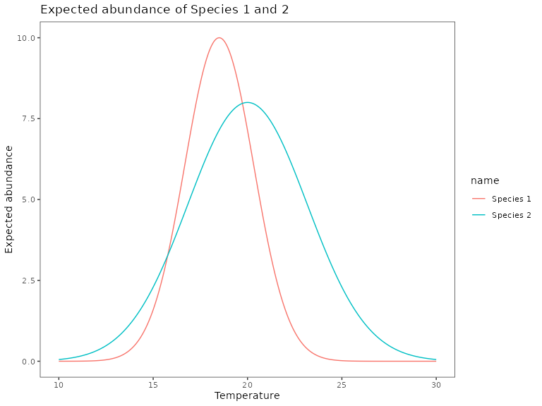

In this simulated landscape, we see that the range of species 1 is much smaller compared to species 2, because it has a much narrower climatic range.

# Baseline occurrences for species 1 and 2
baseline_ab_1 <- rpois_matrix(exp_ab_1(temp, prec))
baseline_ab_2 <- rpois_matrix(exp_ab_2(temp, prec))

baseline_rast <- c(rast(temp), rast(prec), rast(baseline_ab_1), rast(baseline_ab_2))
names(baseline_rast) <- c("Temperature (C)", "Precipitation (mm)", "Abundance (Species 1)", "Abundance (Species 2)")
plot(baseline_rast)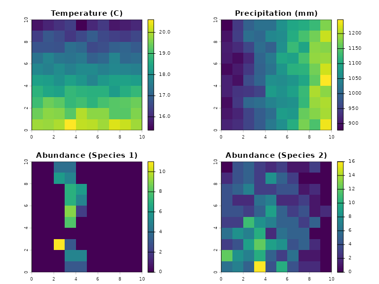

Under future climate change, the temperature and precipitation values are likely to change, resulting in a shift in the range of both species. The scenario modelling community uses a set of standardized scenarios known as the Representative Concentration Pathways (RCPs) or the Shared Socioeconomic Pathways (SSPs) to describe future changes to climate, economic and social variables.

In this simplified example, we demonstrate how Robust Prioritizr can be used to conduct systematic conservation planning when the analyst have predictions of future species ranges across multiple climate scenarios. In this hypothetical example, lets assume that the temperature and precipitation are going to change in the following ways:

SSP1-RCP26: current (baseline) temperature and precipitation values
SSP2-RCP45: mild climate change, temperature increase by 1 degrees Celsius, precipitation reduces by 100mm relative to baseline
SSP4-RCP60: moderate climate change, temperature increase by 2 degrees Celsius, precipitation increases by 50mm on average
SSP5-RCP85: extreme climate change, temperature increase by 3 degrees Celsius, precipitation reduces by 150mm on average

Robust Prioritizr is agnostic to the scenarios that were fed into the model, which means that the analyst is free to specify their own scenarios and names.

In the figure below, we plot the simulated abundances of species 1 and species 2 across these four RCP-SSP pairings. The climatic range of Species 1 in particular is small and is highly sensitive to the future climate scenario. In this case, how can an analyst design a protected area network that accounts for these future changes in climate niches?

plot(abundance_rast)

# Baseline temp and precipitation
temp_ssp1_rcp26 <- temp
prec_ssp1_rcp26 <- prec

# SSP2-RCP45
temp_ssp2_rcp45 <- temp + 1 + matrix(rnorm(N^2, sd = 0.2), N, N)
prec_ssp2_rcp45 <- prec - 100 + matrix(rnorm(N^2, sd = 10), N, N)

# SSP4-RCP60
temp_ssp4_rcp60 <- temp + 2 + matrix(rnorm(N^2, sd = .2), N, N)
prec_ssp4_rcp60 <- prec + 50 + matrix(rnorm(N^2, sd = 10), N, N)

# SSP5-RCP85
temp_ssp5_rcp85 <- temp + 4 + matrix(rnorm(N^2, sd = .2), N, N)
prec_ssp5_rcp85 <- prec - 100 + matrix(rnorm(N^2, sd = 10), N, N)

# Simulate abundance levels given future climates
ssp1_rcp26_ab_1 <- rpois_matrix(exp_ab_1(temp_ssp1_rcp26, prec_ssp1_rcp26))
ssp1_rcp26_ab_2 <- rpois_matrix(exp_ab_2(temp_ssp1_rcp26, prec_ssp1_rcp26))

ssp2_rcp45_ab_1 <- rpois_matrix(exp_ab_1(temp_ssp2_rcp45, prec_ssp2_rcp45))
ssp2_rcp45_ab_2 <- rpois_matrix(exp_ab_2(temp_ssp2_rcp45, prec_ssp2_rcp45))

ssp4_rcp60_ab_1 <- rpois_matrix(exp_ab_1(temp_ssp4_rcp60, prec_ssp4_rcp60))
ssp4_rcp60_ab_2 <- rpois_matrix(exp_ab_2(temp_ssp4_rcp60, prec_ssp4_rcp60))

ssp5_rcp85_ab_1 <- rpois_matrix(exp_ab_1(temp_ssp5_rcp85, prec_ssp5_rcp85))
ssp5_rcp85_ab_2 <- rpois_matrix(exp_ab_2(temp_ssp5_rcp85, prec_ssp5_rcp85))

# Simulate conservation costs
costs <- rnorm(N^2, 100, 20) %>%
  matrix(ncol = N, nrow = N)
costs[matrix(runif(N^2),ncol = N, nrow = N) < 0.05] <- NA # Assume some locked-out constraints

costs_rast <- rast(costs)
names(costs_rast) <- "Cost"

# Group abundances
abundance_rast <- c(
  rast(ssp1_rcp26_ab_1),
  rast(ssp2_rcp45_ab_1),
  rast(ssp4_rcp60_ab_1),
  rast(ssp5_rcp85_ab_1),
  rast(ssp1_rcp26_ab_2),
  rast(ssp2_rcp45_ab_2),
  rast(ssp4_rcp60_ab_2),
  rast(ssp5_rcp85_ab_2)
)

names(abundance_rast) <- c('ssp1_rcp26_ab_1',
                       'ssp2_rcp45_ab_1',
                       'ssp4_rcp60_ab_1',
                       'ssp5_rcp85_ab_1',
                       'ssp1_rcp26_ab_2',
                       'ssp2_rcp45_ab_2',
                       'ssp4_rcp60_ab_2',
                       'ssp5_rcp85_ab_2')

plot(abundance_rast)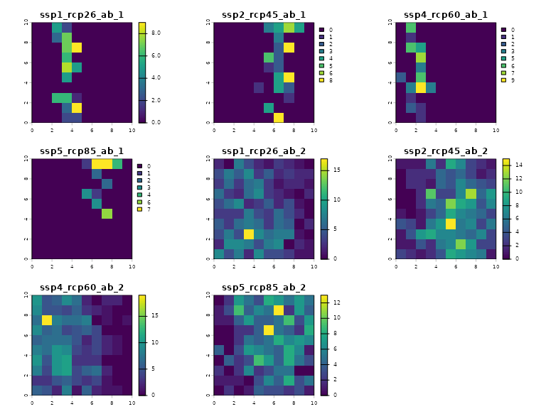

Model specification

We start with a conservation problem where an analyst is tasked with finding the minimum-set protected area network by selecting planning units for protecting two species and ensure that their targets are robust under climate change.

There are many types of uncertainty an analyst can face. Robust Prioritizr is agnostic to the type of uncertainty that is specified, although it is generally useful to be clear on what types of uncertainty exists in a typical systematic conservation planning problem:

Scenario Uncertainty: there are many plausible future scenarios to which features in a planning problem might be affected by
Model Uncertainty: there are different models of ecological systems and conservation costs, or different approaches to modelling ecological systems and costs
Parameter Uncertainty: uncertainty over the specific values of parameters used in the model
Randomness and errors in the model predictions itself

In our first example, we focus mostly on scenario uncertainty, while we will start to build in randomness from the model in the latter parts of the analysis.

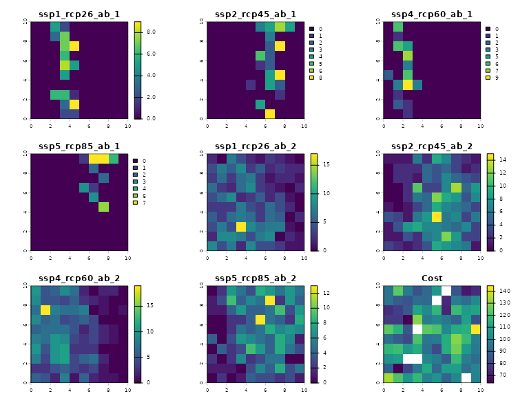
Consider that the analyst has set of predictions of future species abundances for two species under four future RCP-SSP scenarios (SSP1-RCP2.6, SSP2-RCP4.5, SSP4-RCP6.0, and SSP5-RCP8.5), with a specified conservation cost. In the diagram below, we plot the abundance estimates across climate scenarios and its cost:

plot(c(abundance_rast, costs_rast))

The solution identified must satisfy the following constraints:

The total summed abundance of Species 1 within the protected area network must be more than 20 across all planning units across all climate scenarios
The total summed abundance of Species 1 within the protected area network must be more than 20 across all planning units across all climate scenarios
Not select any units with locked-out constraints (Cost = NA)

For simplicity, we do not specify additional constraints, such as connectivity constraints or boundary penalties, in this planning problem.

Solving with standard Prioritizr

As a first pass, we can solve this problem in the traditional Prioritizr specification, using only one of the climate scenarios (SSP2-RCP4.5) for planning. The specification below solves the following conservation planning problem:

\min \sum_{i=1}^{I} x_i c_i

\text{subject to}

\sum_{i=1}^I x_i r_{ij} \geq T_j \quad \forall \space j \in J

x_i \in \{0,1\} \quad \forall \space i \in I

where x is the binary decision variable of whether to protect cell i or not, c is the conservation cost, r is the abundance of species j in cell i (taken as the abundance under SSP2-RCP4.5 at the moment) and T is the representation target for species j (taken as 20 for all species at the moment).

target <- 20
abundance_ssp2_rcp45 <- abundance_rast[[c('ssp2_rcp45_ab_1',
                                         'ssp2_rcp45_ab_2')]]

p1 <- problem(costs_rast, abundance_ssp2_rcp45) %>%
  add_min_set_objective() %>%
  add_absolute_targets(target) %>%
  add_binary_decisions() %>%
  add_default_solver(verbose = F)

s1 <- solve(p1)

plot(s1)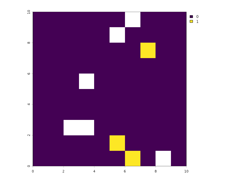

The challenge with this planning approach is that it does not account for other climates. As a result, the planning solution would fail to reach the targets in other climate scenarios, particularly under the extreme climate scenario SSP5-RCP8.5.

plot_solution_eval <- function(soln) {
  representation_rs1 <- values(abundance_rast * soln) %>%
    apply(2, sum, na.rm = T)
  data.frame(value = representation_rs1) %>%
    mutate(name = names(representation_rs1)) %>%
    mutate(name = factor(name, names(representation_rs1), names(representation_rs1))) %>%
    mutate(target_met = if_else(value >= target, 'Target met', 'Target not met')) %>%
    ggplot(aes(x = value, y = name, fill = target_met)) +
    geom_bar(stat = 'identity') +
    geom_vline(xintercept = target) +
    theme_bw() +
    scale_fill_manual(values = c('#0072B2', '#D55E00')) +
    labs(x = 'Abundance in PA', y = '', fill = '') +
    theme(panel.grid = element_blank())
}
plot_solution_eval(s1)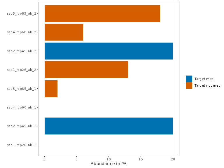

The planning solution identified is not robust to alternative climate scenarios, as the abundance levels within the identified protected area network falls below the target in scenarios other than the selected SSP2-RCP4.5. In particular, it represented almost none of Species 1 under an extreme climate scenario.

Solving with Robust Prioritizr

Robust Prioritizr gives users a flexible interface to solve conservation planning problems that are robust to alternative climate scenarios and other sources of uncertainty. Using the modified minimum set objective, users can solve the following problem:

\min \sum_{i=1}^{I} x_i c_i \text{subject to} \Pr_k \{ \sum_{i=1}^I x_i r_{ijk} \geq T_j \} \geq \alpha \quad \forall \space j \in J x_i \in \{0,1\} \quad \forall \space i \in I

where now r is indexed by k, the feature value for the specific realization (i.e., climate scenario). The problem ensures that the targets are met not just in one specific realization of species abundance, but across many different realizations of scenario k, such that the probability that the targets are met across the realizations exceeds a certain confidence level \alpha. If \alpha=1 (the default and most robust approach), then the solution must meet the species abundance targets across all realizations k and all species j.

Specification of alternative predictions of abundance the same species is achieved through the groups argument of the call to Robust Prioritizr. This enables the user to pass in alternative specifications of the species abundance values in one raster in Prioritizr and tell the problem that these indeed represent the same species/ features across different realizations.

We can extract the relevant groupings from the names of the raster object that we have specified, depending on the specific formatting of the names. These groupings are then supplied to add_*_robust_constraints .

# Recall that the abundance raster is ordered by scenario, then by species,
# i.e. species_1_scenario_1, species_1_scenario_2 etc.
scenario_matrix <- str_split_fixed(names(abundance_rast), pattern = '_', n = 4)
groups <- paste0("species_", scenario_matrix[,4]) # Extract the index in the fourth position
groups

Then, we can solve the problem using Robust Prioritizr, supplying the full raster containing all the abundance predictions across all climate scenarios and the groups argument. For now, we keep the confidence level to 1, ensuring that the targets are met for all species across all scenarios. We can use the robust minimum set objective by invoking add_robust_min_set_objective.

rp1 <- problem(costs_rast, abundance_rast) %>%
  add_constant_robust_constraints(groups = groups) %>%
  add_absolute_targets(target) %>%
  add_robust_min_set_objective() %>%
  add_binary_decisions() %>%
  add_default_solver(verbose = F)

rs1 <- solve(rp1)

s1_combined <- c(s1, rs1)
names(s1_combined) <- c('Non-robust', 'Robust')

plot(s1_combined)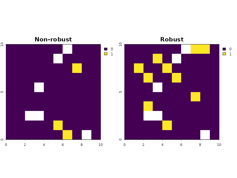

The robust solution identified a lot more planning units compared to the non-robust solution. This is likely because a lot more planning units are needed to ensure that the species ranges are covered across multiple plausible climate scenarios.

We can examine whether the robust solution indeed meets the targets across all of the specified climate scenarios:

plot_solution_eval(rs1)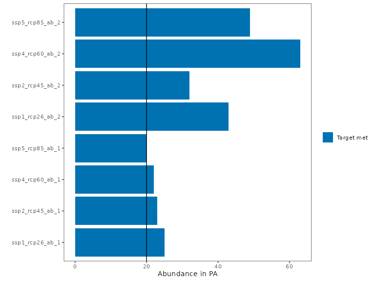

The total abundance in the robust PA network now exceeds the targets in every climate scenario.

Why not just use the worst-case scenario?

The reader is justified in questioning why Robust Prioritizr exists when there could be alternative simple data transformations that the analyst can use to alter the problem to make it appear more conservative. Here we consider three possible approaches and see why these generate a different and inferior solution compared to Robust Prioritizr:

Taking the most extreme climate scenario: the intuition being that if a protected area network meets its target under the most extreme climate scenario, it would be conservative enough to meet the targets in other climate scenarios
Adding a buffer to the target
Taking the minimum values in each planning unit for each species

Taking the most extreme climate scenario

Given in particular the narrow ranges of Species 1, we can see that a protected area network that specifically focuses on protecting its climatic niches under the extreme climate scenario (SSP5-RCP8.5) would still fail to meet its targets under a milder climate scenario. Protecting species with narrow climate niches like Species 1 requires a planning solution that jointly considers all, not just one, climate scenario.

abundance_ssp5_rcp85 <- abundance_rast[[c('ssp5_rcp85_ab_1',
                                         'ssp5_rcp85_ab_2')]]
p2a <- problem(costs_rast, abundance_ssp5_rcp85) %>%
  add_min_set_objective() %>%
  add_absolute_targets(target) %>%
  add_binary_decisions() %>%
  add_default_solver(verbose = F)

s2a <- solve(p2a)

plot_solution_eval(s2a)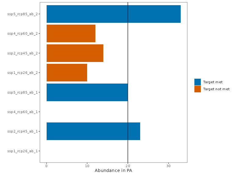

Adding a buffer to the target

Increasing targets might appear to be an easy fix, but it does not account for the reality that the area with abundant species under one climate scenario is not the same as the area with abundant species under a different climate scenario. Thus, increasing the target is only going to select more planning units in areas that are predicted to have an abundant number of species under one climate scenario, while failing to represent the same species under an alternative climate scenario. As a simple demonstration, we see that even multiplying the target by 3 does not solve the problem.

p2b <- problem(costs_rast, abundance_ssp2_rcp45) %>%
  add_min_set_objective() %>%
  add_absolute_targets(target * 3) %>%
  add_binary_decisions() %>%
  add_default_solver(verbose = F)

s2b <- solve(p2b)

plot_solution_eval(s2b)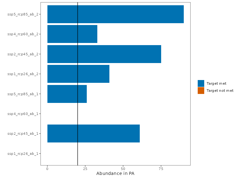

Taking the minimum value across scenarios

A common misconception to why robust optimization does under the hood (one that I had in the past) was that solving a problem with a robust approach is equivalent to solving the problem while supplying the minimum value of the abundance across all scenarios. Such approaches are common in so-called “climate refugia” analyses, where the objective is to identify overlaps in species ranges across multiple climate scenarios and direct conservation efforts to those areas.

For example, we can identify areas where Species 2 (the species with broader climatic niches) are present in the dataset by taking the minimum of the abundance estimates across climate scenarios:

abundance_min_2 <- c(abundance_rast[[5]] > 0,
                   abundance_rast[[8]] > 0,
                   min(abundance_rast[[5:8]] > 0))
abundance_min_2 %>% plot()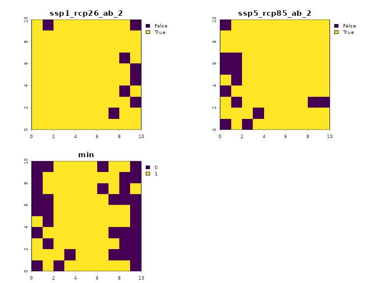

In this case, we see that there are still some overlap in species ranges across climate scenarios. If we use the minimum to represent the abundance for species 2, we can solve the problem, but still see that the solution that it identifies becomes too conservative, with the abundance levels exceeding the target by a substantial margin (leading to higher costs).

abundance_min <- abundance_ssp2_rcp45
abundance_min[[2]] <- min(abundance_rast[[5:8]]) # Only set that for species 2
p2c <- problem(costs_rast, abundance_min) %>%
  add_min_set_objective() %>%
  add_absolute_targets(target) %>%
  add_binary_decisions() %>%
  add_default_solver(verbose = F)
s2c <- solve(p2c)
plot_solution_eval(s2c)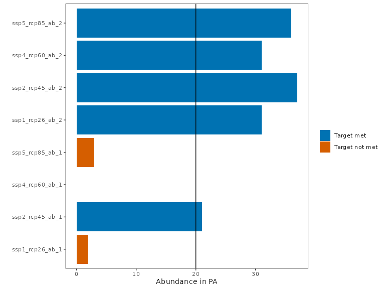

In some cases, such an analysis may not even yield feasible solutions. For example, consider Species 1, where its ranges do not overlap at all across climate scenarios. Taking the minimum out of abundance estimates of all scenarios would lead to a minimum value of zero abundance for all planning units. If these features were used for prioritization, the problem would be infeasible. As seen in the figure below, the minimum value of the abundance levels are all zero in all planning units.

abundance_min_1 <- c(abundance_rast[[1]] > 0,
                   abundance_rast[[4]] > 0,
                   min(abundance_rast[[1:4]] > 0))
abundance_min_1 %>% plot(type = 'continuous', range = c(0,1))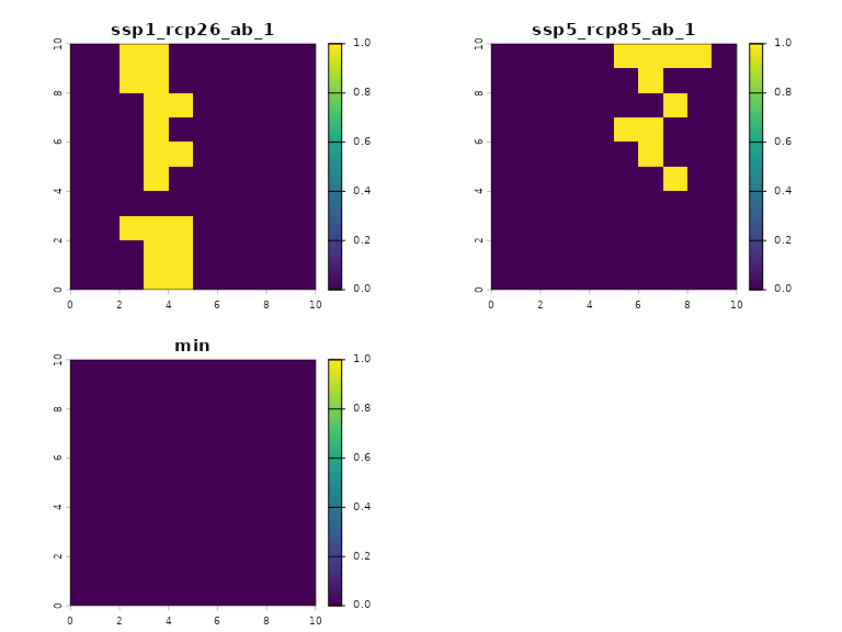

Tuning the level of robustness

The confidence level parameter conf_level gives users the flexibility to alter the level of robustness in the solution. This parameter is interpreted as the minimum proportion of realizations (out of the total number of realizations) for which the target is satisfied. By default, the target needs to be met across all realizations (conf_level=1). In some cases, relaxing the conf_level parameter to something less than 1 can help the solver find a solution that has a higher objective value, or turns it from an infeasible problem to a feasible one.

The more realizations we have in the problem, the more meaningful it is for the user to specify a conf_level less than 1. This is because, say we have a problem with only 4 realizations of uncertainty (4 scenarios). For the conf_level parameter to have any effect on the solution, it has to be lower than 0.75, where the target can be violated in at least 1 out of the 4 realizations. Anything higher than 0.75 will not affect the model.

Now consider the case where a user has something like more than 100 realizations of data, say it is drawn from a statistical distribution. The parameter then becomes much more meaningful. Tuning the confidence level parameter to something like 0.95 means that the target is met across 95% (or 95 out of 100) of the realizations, ensuring that the constraint is held in a large proportion of realizations and guaranteeing solution quality while giving some flexibility for the problem to search for better solutions.

To demonstrate how the confidence level parameter works, we build in additional uncertainty to our existing problem. Recall that the abundance estimates we have are from a statistical model that is estimated with uncertainty. Consider a matrix of coefficients beta_species_dist_* that carries the uncertainty of the parameters describing the relationship between temperature, precipitation and expected abundance. We can then use that distribution of parameters to draw species abundance across the scenarios we have. We consider a small example with a total of 40 realizations of uncertainty in this problem, with n_replicates replicates for each climate scenario.

n_replicates <- 10

# Simulate abundance levels given future climates
ssp1_rcp26_ab_1 <- replicate(n_replicates, ab_draw_pois(temp_ssp1_rcp26, prec_ssp1_rcp26, beta_species_dist_1))
ssp1_rcp26_ab_2 <- replicate(n_replicates, ab_draw_pois(temp_ssp1_rcp26, prec_ssp1_rcp26, beta_species_dist_2))

ssp2_rcp45_ab_1 <- replicate(n_replicates, ab_draw_pois(temp_ssp2_rcp45, prec_ssp2_rcp45, beta_species_dist_1))
ssp2_rcp45_ab_2 <- replicate(n_replicates, ab_draw_pois(temp_ssp2_rcp45, prec_ssp2_rcp45, beta_species_dist_2))

ssp4_rcp60_ab_1 <- replicate(n_replicates, ab_draw_pois(temp_ssp4_rcp60, prec_ssp4_rcp60, beta_species_dist_1))
ssp4_rcp60_ab_2 <- replicate(n_replicates, ab_draw_pois(temp_ssp4_rcp60, prec_ssp4_rcp60, beta_species_dist_2))

ssp5_rcp85_ab_1 <- replicate(n_replicates, ab_draw_pois(temp_ssp5_rcp85, prec_ssp5_rcp85, beta_species_dist_1))
ssp5_rcp85_ab_2 <- replicate(n_replicates, ab_draw_pois(temp_ssp5_rcp85, prec_ssp5_rcp85, beta_species_dist_2))

To fit this into Robust Prioritizr, we bring these replicates into 1 single multilayer raster.

species_1_realizations <- c(rast(ssp1_rcp26_ab_1),
                            rast(ssp2_rcp45_ab_1),
                            rast(ssp4_rcp60_ab_1),
                            rast(ssp5_rcp85_ab_1))
names(species_1_realizations) <- c(paste0("s1_ssp1_rcp26_r", 1:n_replicates),
                                   paste0("s1_ssp2_rcp45_r", 1:n_replicates),
                                   paste0("s1_ssp4_rcp60_r", 1:n_replicates),
                                   paste0("s1_ssp5_rcp85_r", 1:n_replicates))

species_2_realizations <- c(rast(ssp1_rcp26_ab_2),
                            rast(ssp2_rcp45_ab_2),
                            rast(ssp4_rcp60_ab_2),
                            rast(ssp5_rcp85_ab_2))
names(species_2_realizations) <- c(paste0("s2_ssp1_rcp26_r", 1:n_replicates),
                                   paste0("s2_ssp2_rcp45_r", 1:n_replicates),
                                   paste0("s2_ssp4_rcp60_r", 1:n_replicates),
                                   paste0("s2_ssp5_rcp85_r", 1:n_replicates))

abundance_uncertainty <- c(species_1_realizations, species_2_realizations)
groups_uncertainty <- c(rep("s1", n_replicates*4),
                        rep("s2", n_replicates*4))

Here we solve the problem without altering the confidence level. If we do not alter the confidence level parameter, we can expect the target to be met across all planning units.

rp2a <- problem(costs_rast, abundance_uncertainty) %>%
  add_constant_robust_constraints(groups = groups_uncertainty) %>%
  add_absolute_targets(target) %>%
  add_robust_min_set_objective() %>%
  add_binary_decisions() %>%
  add_default_solver(verbose = F)

rs2a <- solve(rp2a)

Fortunately, a solution can be found. We can see that the target is met across all of the replicates we provide to the problem.

eval_soln_uncertain <- function(soln, return_df = FALSE) {
  dist <- values(soln * abundance_uncertainty) %>%
    unname %>%
    apply(2, sum, na.rm = T)
  df <- data.frame(groups = groups_uncertainty, value = dist) %>%
    mutate(target_met = if_else(value >= target, 'Target met', 'Target not met'))
  if (return_df) return(df)
  df %>%
    ggplot(aes(x = value, fill = target_met)) +
    geom_histogram() +
    geom_vline(xintercept = target) +
    facet_wrap(vars(groups), ncol = 1) +
    scale_fill_manual(values = c('#0072B2', '#D55E00')) +
    theme_bw() +
    theme(panel.grid = element_blank())
}
eval_soln_uncertain(rs2a)

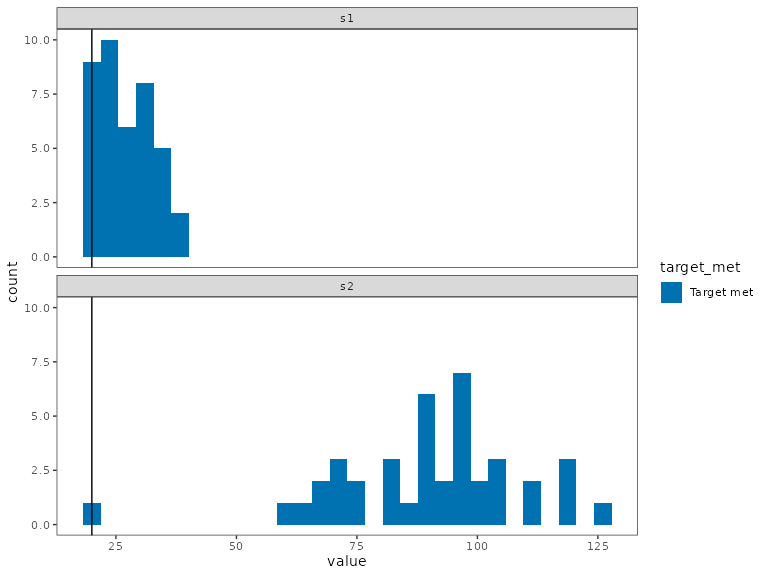
As the number of replicates increase, it becomes increasingly hard for the problem to find feasible solutions. It also increases the cost of the solution.

If we relax the confidence level a bit, we can allow for the target to not be met in some realizations of uncertainty. This allows the optimisation problem to search for a lower cost solution. For example, we can specify the conf_level=0.9, which mandates that the solution meet the objective in at least 90% of the random realizations supplied to the problem.

# Note that "method = 'chance'" may not be scalable to larger problems
rp2b <- problem(costs_rast, abundance_uncertainty) %>%
  add_constant_robust_constraints(groups = groups_uncertainty, conf_level = .9) %>%
  add_absolute_targets(target) %>%
  add_robust_min_set_objective(method = 'chance') %>%
  add_binary_decisions() %>%
  add_default_solver(verbose = F)

rs2b <- solve(rp2b)

eval_soln_uncertain(rs2b)

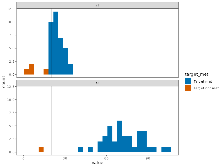
We see that the proportion of the targets that were met are all at least 90%. For Species 2, as it has a much wider representation in the landscape, the conservation target is met in much more than 90% of the replicates.

eval_soln_uncertain(rs2b, return_df = TRUE) %>%
  group_by(groups) %>%
  summarise(prop_target_met = mean(target_met == 'Target met') )

Users can also evaluate the relative trade-offs between robustness and the costs of the solutions identified by examining the trade-off curve across different confidence level specifications.

conf_level_vect <- seq(0.5, 1, 0.1)
solve_chance_cons <- function(c) {
                 p <- problem(costs_rast, abundance_uncertainty) %>%
                  add_constant_robust_constraints(groups = groups_uncertainty, conf_level = c) %>%
                  add_absolute_targets(target) %>%
                  add_robust_min_set_objective(method = 'chance') %>%
                  add_binary_decisions() %>%
                  add_default_solver(verbose = F)
                 solve(p)
               }

rp2c <- list()
solve_times <- c()
for (i in 1:length(conf_level_vect)) {
  start.time <- Sys.time()
  rp2c[[i]] <- solve_chance_cons(conf_level_vect[i])
  end.time <- Sys.time()
  solve_times <- c(solve_times, end.time - start.time)
}


sp2c <- rast(rp2c)
cost_conf_level <- values(sp2c * costs_rast) %>%
  apply(2, sum, na.rm = T)

chance_cons_df <- data.frame(conf_level = conf_level_vect, cost = cost_conf_level, solve_times)

chance_cons_df %>%
  ggplot(aes(x = conf_level, y = cost)) +
  geom_point() +
  geom_line() +
  scale_x_reverse() +
  theme_bw() +
  labs(x = 'Confidence Level', y = 'Cost') +
  theme(panel.grid = element_blank())

Do however note that the setting of conf_level to anything other than 1 will increase the solve times and can make your problem intractable for a large number of planning units/ realizations.

chance_cons_df %>%
  ggplot(aes(x = conf_level, y = solve_times)) +
  geom_point() +
  geom_line() +
  scale_x_reverse() +
  theme_bw() +
  labs(x = 'Confidence Level', y = 'Solve times', title = "Solve times using Chance Constraints (Gurobi)") +
  theme(panel.grid = element_blank())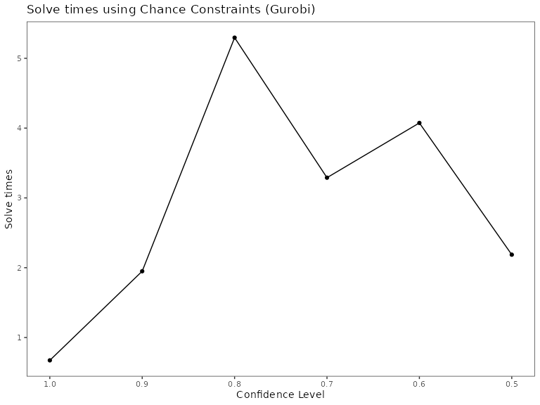

Users should carefully evaluate whether it is necessary to adjust the conf_level parameter and understand the consequences it can have for solving larger problems.