Add robust minimum set objective

Add an objective to a conservation planning problem that minimizes the cost of the solution while ensuring that the solution is robust to uncertainty for each feature group.

Usage

add_robust_min_set_objective(x, method = "chance")

Arguments

x: prioritizr::problem() object.
method: character value with the name of the probabilistic constraint formulation method. Available options include the ("chance") chance constraint programming method (Charnes and Cooper 1959) or ("cvar") or the conditional value-at-risk method (Rockafellar and Uryasev 2000), Defaults to "chance". See the Details section for further information on these methods.

Value

An updated prioritizr::problem() object with the objective added to it.

Details

The robust minimum set objective seeks to find the set of planning units at a minimum cost such that the solution meets the targets in a robust manner for each feature group. Two methods are provided for formulating the optimization problem as a mixed integer linear programming problem. These methods are the chance constraint programming method (method = "chance") and conditional value-at-risk method (method = "cvar"). In particular, the chance constraint programming method is associated a more intuitive interpretation for the confidence level parameter (i.e., specified per conf_level with add_constant_robust_constraints() or add_variable_robust_constraints()). Whereas, the conditional value-at-risk constraint method may yield faster solve times. This is because the conditional value-at-risk constraint method preserves the convexity of an optimization problem, and uses continuous (instead of binary) auxiliary variables. Also note that the conditional value-at-risk constraint method may produce an infeasible solution for problems that are feasible with the chance constraint with the same conf_level. In such cases the chance chance constraint programming method should be used instead. As such, the chance constraint programming method may be more useful for facilitating stakeholder involvement for small-scale planning exercises, and the conditional value-at-risk constraint method may be more useful for large-scale applications.

Mathematical formulation

This objective can be expressed mathematically for a set of planning units ($I$ indexed by $i$), a set of feature groups ($J$ indexed by $j$), and a set of features associated with each feature group ($K$ indexed by $k$). Let $c_i$ denote the cost of planning unit $i$, $r_{ijk}$ the amount of feature $k$ associated with planning unit $i$ for feature group $j$, $T_j$ the target for each feature group $j$, and $\alpha$ the confidence level for uncertainty (specified per conf_level with add_constant_robust_constraints() or add_variable_robust_constraints()). Additionally, to describe the decision variables, let $x_i$ denote the status of the planning unit $i$ (e.g., specifying whether planning unit $i$ has been selected or not with binary values). Given this terminology, the robust minimum set formulation of the reserve selection problem is formulated as follows.

$$ \mathit{Minimize} \space \sum_{i = 1}^{I} x_i c_i \\ \mathit{subject \space to} \\ \Pr_k \{ \sum_{i = 1}^{I} x_i r_{ijk} \geq T_j \} \geq \alpha \quad \forall \space j \in J $$

Here, the objective function (first equation) is to minimize the total cost of the solution. The probabilistic constraints (second equation) specify that the solution must achieve a particular probability threshold (based on $\alpha$) for meeting the targets of the features associated with each feature group. For example, if $\alpha=1$, then each and every target associated with each feature group must be met. Alternatively, if $\alpha=0.5$, then the solution must have a 50% chance of meeting the targets associated with each feature group. Approximation methods are used to linearize them so that the optimization problem can be solved with mixed integer programming exact algorithm solvers.

The chance constraint programming method uses a "big-M" formulation to linearize the probabilistic constraints (Charnes and Cooper 1959). To describe this method, let $m_{jk}$ denote a binary auxiliary variable for each feature $k$ associated with each feature group $j$. Also, let $K_j$ denote a pre-computed value describing the number of features associated with each feature group $j$. Given this terminology, the method involves replacing the probabilistic constraints with the following linear constraints.

$$ \sum_{i = 1}^{I} x_i r_{ijk} + T_j m_{jk} \geq T_{j} \quad \forall \space j \in J, \space k \in K \\ \sum_{k = 1}^{K_j} \frac{m_{jk}}{K_j} \leq 1 - \alpha \quad \forall \space j \in J \\ m_{jk} \in \{0, 1\} \quad \forall \space j \in J, \space k \in K $$

Here, the solution is allowed to fail to meet the targets for the features, and the auxiliary variable $m_{jk}$ is used to calculate the proportion of features that do not have their targets met for each feature group. For a given feature group, the proportion of features that do not have their target met is constrained to be less than $1 - \alpha$. This method allows for an intuitive interpretation of the confidence level parameter. Yet this method also adds $J \times K$ binary variables to the problem and, as such, may present long solve times for problems with many other decision variables and constraints.

The conditional value-at-risk constraint method presents a tighter formulation than the chance constraint programming method (Rockafellar and Uryasev 2000). As such, this method is able to better approximate the probabilistic constraints and, in turn, could potentially yield solutions that are more robust to uncertainty and less cost-efficient than the chance constraint programming method. To describe this method, let $\eta_j$ denote a continuous auxiliary variable for each feature group $j$, and $s_{jk}$ a continuous auxiliary variable for each feature $k$ associated with each feature group $j$. Given this terminology, the method involves replacing the probabilistic constraints with the following linear constraints.

$$ \sum_{i = 1}^{I} x_i r_{ijk} - \eta_j + s_{jk} \geq 0 \quad \forall \space j \in J, \space k \in K \\ \eta_j - \frac{1}{(1 - \alpha) \times K_j} \sum_{k=1}^{K_j} s_{jk} \geq T_j \quad \forall \space j \in J \\ s_{jk} \geq 0 \quad \forall \space j \in J, \space k \in K \\ \eta_j \in \mathbb{R} \quad \forall \space j \in J $$

Here, the continuous auxiliary variables are used to represent the "tail" of the distribution of the uncertain quantity (i.e., $\sum_{i=1}^{I} x_i r_{ijk}$). In other words, it ensures that the average of amount of each feature held by the solution for a particular feature group that falls below a particular quantile (i.e., $(1 - \alpha)$) is greater than the target for the feature group (i.e., $T_j$). Although this method does not provide an easily intuitive interpretation of the confidence level parameter, it only adds $J \times K + J$ continuous variables to the problem.

References

Charnes A & Cooper WW (1959) Chance-constrained programming. Management Science, 6(1), 73–79.

Rockafellar RT & Uryasev S (2000) Optimization of conditional value-at-risk. Journal of Risk, 2(3), 21–42.

Examples

if (FALSE) { # \dontrun{
# Load packages
library(prioritizr)
library(terra)

# Get planning unit data
pu <- get_sim_pu_raster()

# Get feature data
features <- get_sim_features()

# Define the feature groups,
# Here, we will assign the first 2 features to the group A, and
# the remaining features to the group B
groups <- c(rep("A", 2), rep("B", nlyr(features) - 2))

# Build problem with chance constraint programming method
p <-
  problem(pu, features) |>
  add_robust_min_set_objective(method = "cvar") |>
  add_constant_robust_constraints(groups = groups, conf_level = 0.9) |>
  add_binary_decisions() |>
  add_relative_targets(0.1) |>
  add_default_solver(verbose = FALSE)

# Solve the problem
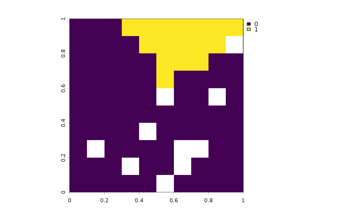
soln <- solve(p)

# Plot the solution
plot(soln)
} # }