5. Risk preferences: elicitation, sensitivity, and validation
Source:vignettes/vira-05-elicitation.Rmd
vira-05-elicitation.RmdThe previous vignettes computed VOI for a fixed risk-aversion level. In practice the decision-maker’s risk preference is unknown — it must be elicited through a structured sequence of questions. This introduces its own uncertainty: the elicitation returns a distribution over plausible values of the risk parameter, not a single number. That uncertainty then propagates into the VOI estimate.
This vignette follows the full workflow in order:
- Elicitation — how to query a decision-maker and represent their risk preference.
- Sensitivity — how VOI varies across the elicitation posterior, and why the point-estimate answer may differ from the posterior-weighted answer.
- Validation — how accurate the elicitation algorithm actually is, assessed by replacing the human with a simulated agent of known preferences.
Part 1 — Eliciting risk preferences
Why risk preferences matter for VOI
When you calculate the Value of Information, the answer depends on how the decision-maker feels about uncertainty. Two managers facing the same frog conservation problem might place very different value on learning more — if one is deeply averse to the possibility of a bad outcome, they will pay more to resolve uncertainty than someone who simply wants to maximise the average.
The risk preference captures this: a single number summarising how much someone dislikes uncertainty, on a scale from strongly risk-seeking (happy to gamble) to strongly risk-averse (willing to pay a premium for certainty).
How the elicitation works
vira asks the decision-maker a series of simple choice
questions. Each question presents two options:
- Option A — a gamble: a high outcome with some probability, and a low outcome otherwise.
- Option B — a sure thing: a fixed outcome for certain.
The certain amount in Option B is set so that, under the current best guess of the decision-maker’s risk preference, they should be roughly indifferent between A and B. If they choose A, they are more risk-seeking than assumed; if they choose B, they are more risk-averse. After each answer, the algorithm narrows its estimate. After around 8–12 questions, the estimate has usually converged.
This approach is called Bayesian adaptive elicitation: the algorithm maintains a probability distribution over all plausible risk aversion values and updates it after each answer using Bayes’ rule.
D-efficient question design
Not all questions are equally informative. A question is maximally useful when its answer shifts the posterior as much as possible — technically, when it maximises the expected Fisher information under the current posterior.
vira uses a Bayesian D-efficient design criterion
(following Jonker & Bliemer 2019): before each question, it searches
over candidate outcome ranges and picks the one that maximises
where the sum is over the discretised posterior (weights ), is the probability of choosing Option B under a logit model with scale , and is the sensitivity of the normalised certainty-equivalent utility to the risk parameter. The EFI is evaluated on a coarse subgrid for speed, with the final outcome range then used to construct the next question.
Running the elicitation
In a real session, call elicit_risk_preferences() and
answer the questions in the console:
rp <- elicit_risk_preferences(
  outcome_name = "frogs",
  val_min      = 0,
  val_max      = 200,
  maximize     = TRUE
)
The function returns a risk_preference object and plots
the posterior distribution over the risk parameter together with the
implied utility curve.
Using a known parameter
If the risk aversion value is already known (from a prior study or an expert panel), construct the object directly:
rp <- risk_preference(
  model        = "CRRA",
  param        = 1.5,
  val_min      = 0,
  val_max      = 200,
  outcome_name = "frogs",
  maximize     = TRUE
)
rp
What does model = "CRRA" mean?
You do not need to remember the name (Constant Relative Risk Aversion). It describes a common pattern: each additional gain matters a little less than the last one. Saving the first 10 frogs feels more important than saving frog number 191 through 200.
The param argument controls the strength of this
effect:
-
param = 0— risk-neutral: every frog counts equally. -
param = 1— mildly risk-averse: earlier gains matter more. -
param = 3— strongly risk-averse: strongly prioritise avoiding very bad outcomes, even at the cost of a lower average.
The alternative model "CARA" (Constant Absolute Risk
Aversion) behaves similarly but is more appropriate when outcomes are
costs rather than counts (e.g., dollars lost).
What the utility curve looks like
The utility curve shows how much each additional frog is “worth” to
the decision-maker. Under risk aversion, each extra frog is worth a
little less than the previous one — the curve bends downward. A higher
param value means stronger risk aversion and a more
pronounced bend.
par(mfrow = c(1, 3), mar = c(4, 4, 2, 1))
for (g in c(0.5, 1.5, 3)) {
  rp_tmp <- risk_preference("CRRA", param = g, val_min = 0, val_max = 200,
                             outcome_name = "frogs", maximize = TRUE)
  plot(rp_tmp, main = paste("gamma =", g))
}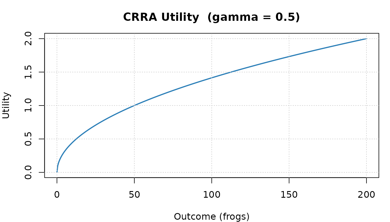
Utility curves for three levels of risk aversion.
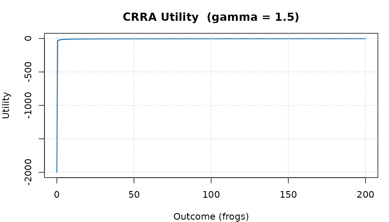
Utility curves for three levels of risk aversion.
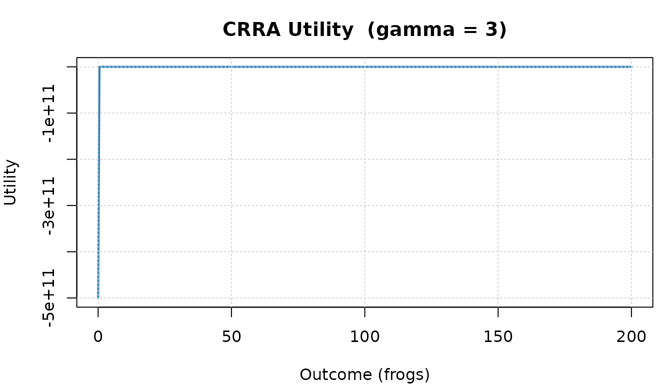
Utility curves for three levels of risk aversion.
Turning the preference into a utility function
To use the elicited preference in a VOI calculation, call
use_risk_preference(). This returns a list with two
functions — utility and inv_utility — ready to
plug into the pipe:
rp  <- risk_preference("CRRA", param = 1, val_min = 0, val_max = 200,
                        outcome_name = "frogs", maximize = TRUE)
fns <- use_risk_preference(rp)

frog_counts <- c(55, 100, 135, 200)
fns$utility(frog_counts)
#> [1] -1.2909815 -0.6931462 -0.3930421  0.0000000
fns$inv_utility(fns$utility(frog_counts))  # round-trips back to frogs
#> [1]  55 100 135 200
The inv_utility function converts utility values back to
frog counts, which is how VOI ends up expressed in the original outcome
units.
Part 2 — VOI is sensitive to the elicited preference
The elicitation returns a distribution, not a number
A real elicitation session does not return a single gamma value — it returns a posterior distribution over all plausible values. The mean of that posterior is the best point estimate, but the spread quantifies how much uncertainty remains after the questions were answered.
That uncertainty matters because the VOI curve is often nonlinear in gamma: a small shift in the estimated risk parameter can noticeably change the computed VOI. Propagating the elicitation posterior through the VOI calculation turns a single VOI number into a credible interval — telling the decision-maker not just “VOI = 12 frogs” but “VOI is somewhere between 9 and 16 frogs, depending on how risk-averse you actually are.”
Setup: chytrid EVPI problem with elicitation posterior
We use the Canessa et al. (2015) chytrid problem from vignettes 1–2. We simulate what a real elicitation posterior might look like: centred on gamma = 1 with standard deviation ≈ 0.6, representing moderate spread after roughly 8–10 questions.
data("canessa2015")
problem <- voi_problem(canessa2015$V, canessa2015$p)
set.seed(42)
grid    <- seq(-1, 4, length.out = 800)
raw     <- dnorm(grid, mean = 1, sd = 0.6)
weights <- raw / sum(raw)

rp_elicited <- risk_preference(
  model        = "CRRA",
  param        = sum(grid * weights),       # posterior mean
  param_ci     = c(
    grid[which(cumsum(weights) >= 0.025)[1]],
    grid[which(cumsum(weights) >= 0.975)[1]]
  ),
  posterior    = list(grid = grid, weights = weights),
  val_min      = 0,
  val_max      = 200,
  outcome_name = "frogs",
  maximize     = TRUE
)

cat("Posterior mean gamma:", round(rp_elicited$param, 3), "\n")
#> Posterior mean gamma: 1.001
cat("95% CI: [",
    round(rp_elicited$param_ci[1], 3), ",",
    round(rp_elicited$param_ci[2], 3), "]\n")
#> 95% CI: [ -0.174 , 2.179 ]
Running the sensitivity sweep
voi_sensitivity() recomputes VOI across the full
posterior grid and returns a data frame with the posterior weight for
each gamma value:
sens <- voi_sensitivity(problem, rp_elicited)
head(sens)
#>        param      voi posterior_weight is_posterior_mean
#> 1 -1.0000000 15.71842     1.609229e-05             FALSE
#> 2 -0.9937422 15.75623     1.666069e-05             FALSE
#> 3 -0.9874844 15.79411     1.724728e-05             FALSE
#> 4 -0.9812265 15.83205     1.785258e-05             FALSE
#> 5 -0.9749687 15.87007     1.847712e-05             FALSE
#> 6 -0.9687109 15.90814     1.912142e-05             FALSE
VOI curve with posterior uncertainty
mean_voi <- sum(sens$voi * sens$posterior_weight, na.rm = TRUE)

ord     <- order(sens$voi)
cdf_voi <- cumsum(sens$posterior_weight[ord])
voi_lo  <- sens$voi[ord][which(cdf_voi >= 0.025)[1]]
voi_hi  <- sens$voi[ord][which(cdf_voi >= 0.975)[1]]

plot(sens$param, sens$voi,
     type = "n",
     xlab = "Risk aversion (gamma)",
     ylab = "EVPI (frogs)",
     main = "Sensitivity of EVPI to elicited risk preference",
     ylim = c(0, max(sens$voi, na.rm = TRUE) * 1.15))

polygon(
  c(sens$param, rev(sens$param)),
  c(sens$voi * (sens$posterior_weight / max(sens$posterior_weight)) * 0 +
      min(sens$voi, na.rm = TRUE),
    rev(sens$voi)),
  col = adjustcolor("#2c7fb8", alpha.f = 0.15), border = NA
)

lines(sens$param, sens$voi, lwd = 2, col = "#2c7fb8")
abline(v = rp_elicited$param, lty = 2, col = "grey30")
abline(h = mean_voi, lty = 3, col = "#e34a33")

legend("topright",
       legend = c("VOI curve", "Posterior mean gamma",
                  sprintf("Posterior-weighted VOI = %.1f frogs", mean_voi)),
       lty    = c(1, 2, 3),
       col    = c("#2c7fb8", "grey30", "#e34a33"),
       lwd    = c(2, 1, 1),
       bty    = "n", cex = 0.85)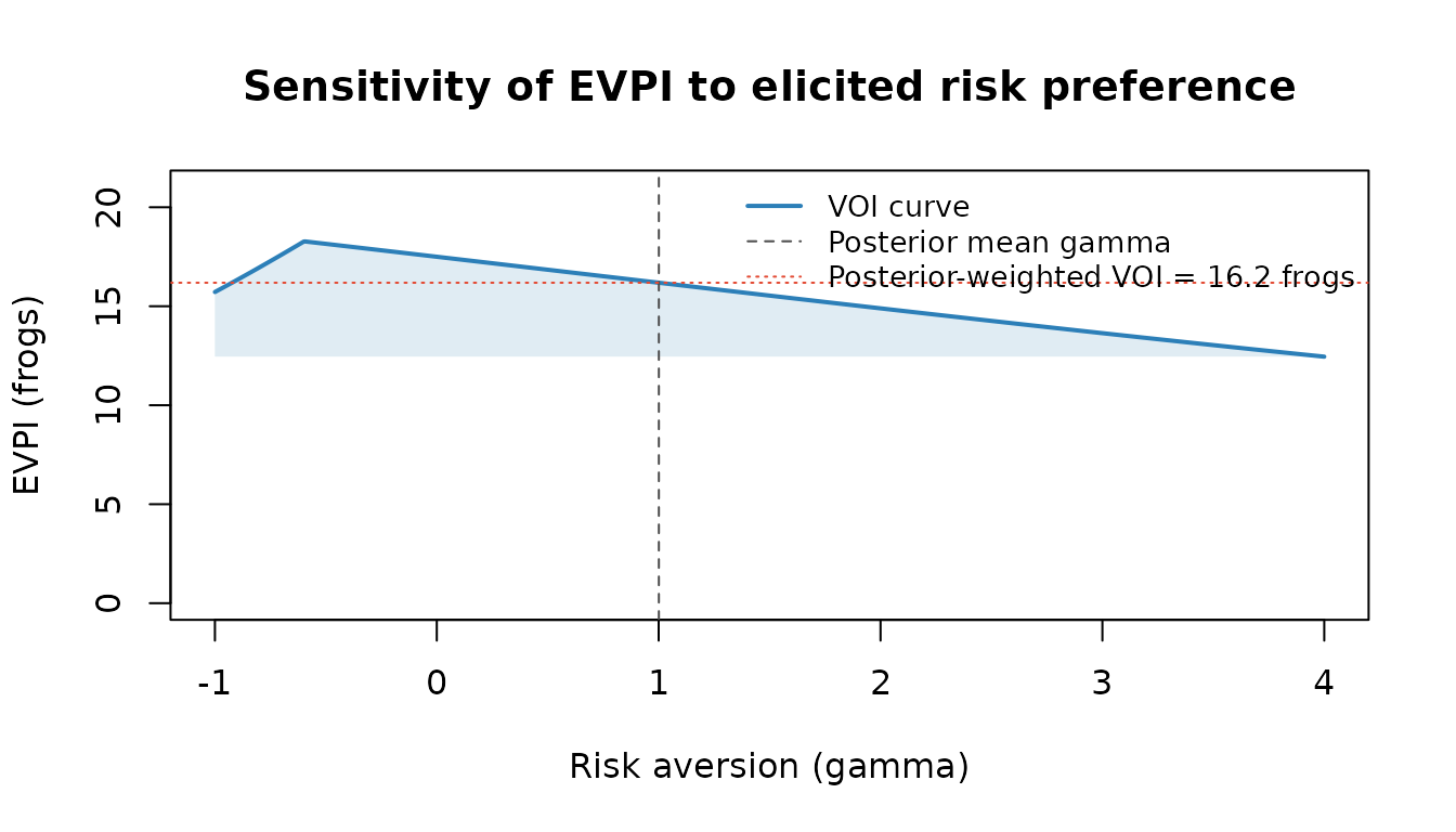
VOI as a function of risk aversion. The shaded band represents the posterior density from the elicitation; the horizontal dashed line is the posterior-weighted expected VOI.
Summarising the posterior VOI distribution
cat("VOI at posterior mean:       ", round(sens$voi[sens$is_posterior_mean], 2), "\n")
#> VOI at posterior mean:        16.19
cat("Posterior-weighted mean VOI: ", round(mean_voi, 2), "\n")
#> Posterior-weighted mean VOI:  16.19
cat("95% credible interval:       [", round(voi_lo, 2), ",", round(voi_hi, 2), "]\n")
#> 95% credible interval:       [ 14.67 , 17.69 ]
The difference between the VOI at the point estimate and the posterior-weighted mean reflects Jensen’s inequality: if the VOI curve is nonlinear (concave or convex in gamma), integrating over the posterior shifts the answer relative to the point estimate alone.
Where does uncertainty in gamma matter most?
dvoi <- diff(sens$voi) / diff(sens$param)
plot(sens$param[-1], dvoi, type = "l", lwd = 2, col = "#7f3b08",
     xlab = "Risk aversion (gamma)",
     ylab = "dVOI / d(gamma)",
     main = "Where does elicitation uncertainty matter most?")
abline(h = 0, lty = 3, col = "grey60")
abline(v = rp_elicited$param, lty = 2, col = "grey30")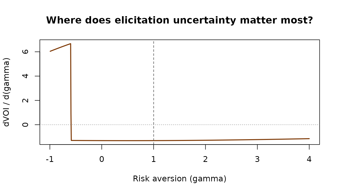
The gradient of VOI with respect to gamma. Where the slope is steep, elicitation error translates directly into VOI error.
Where the gradient is steep, a small error in the elicited gamma will change the VOI substantially. Where the gradient is flat, the VOI is robust to elicitation uncertainty. The gradient plot therefore tells you which part of the elicitation to invest in refining — if the posterior mean sits on a steep slope, more questions are worth asking.
Part 3 — How accurate is the elicitation algorithm?
How many questions are needed?
The sensitivity analysis above shows that elicitation uncertainty propagates into VOI uncertainty. The natural next question is: how much uncertainty does the algorithm actually leave, and how quickly does it converge?
The simulation below replaces the human respondent with a robot agent — a simulated decision-maker whose true risk parameter is known. It measures mean absolute error (MAE) between the true and recovered parameter as a function of the number of questions asked.
set.seed(42)
acc <- run_accuracy_vs_questions(
  q_range          = 1:16,
  param_values     = seq(-1.5, 3.5, by = 1),
  trials_per_param = 10
)

plot(acc$n_questions, acc$mae, type = "b", pch = 19,
     col = "#2c3e50", lwd = 2,
     xlab = "Number of questions", ylab = "Mean absolute error (risk parameter)",
     main = "Elicitation accuracy vs number of questions",
     ylim = c(0, max(acc$mae) * 1.05), las = 1)
grid(lty = 3, col = "grey80")
abline(h = min(acc$mae) * 1.2, lty = 2, col = "#e74c3c", lwd = 1.5)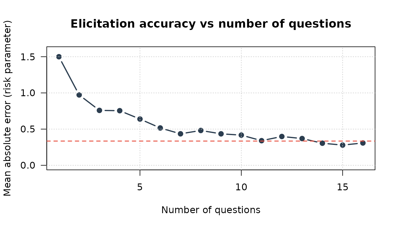
MAE in recovered risk parameter falls rapidly with additional questions and levels off around 8–10 questions.
The sharp initial drop reflects the high information content of the
first few D-efficient questions; returns diminish beyond about 8
questions for most practical purposes. The default of
max_questions = 12 leaves a comfortable margin above this
knee in the curve.
Robot calibration across parameter values
To assess accuracy across the full range of risk preferences, we run 20 robot sessions at each of 17 true gamma values, then compare the inferred parameter to the true value:
set.seed(2025)
results <- run_asymptotic_performance_suite(
  param_values     = seq(-1.5, 3.5, by = 0.5),
  trials_per_param = 20,
  model            = "CRRA",
  val_min          = 0,
  val_max          = 120
)
#> === vira Elicitation Calibration Suite ===
#> Model: CRRA | 11 params x 20 trials
#>
#>   gamma = -1.50 MAE = 0.2907
#>   gamma = -1.00 MAE = 0.3135
#>   gamma = -0.50 MAE = 0.3557
#>   gamma = +0.00 MAE = 0.2714
#>   gamma = +0.50 MAE = 0.2466
#>   gamma = +1.00 MAE = 0.2993
#>   gamma = +1.50 MAE = 0.4588
#>   gamma = +2.00 MAE = 0.3090
#>   gamma = +2.50 MAE = 0.3560
#>   gamma = +3.00 MAE = 0.4680
#>   gamma = +3.50 MAE = 0.3078
#>
#> Global MAE: 0.3342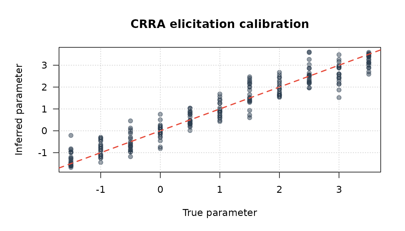
plot(results$True_Param, results$Inferred_Mean,
     pch  = 19,
     col  = adjustcolor("#2c7fb8", alpha.f = 0.4),
     xlab = "True risk parameter (gamma)",
     ylab = "Inferred parameter",
     main = "CRRA elicitation calibration",
     las  = 1)
abline(a = 0, b = 1, col = "#e34a33", lwd = 2, lty = 2)
legend("topleft",
       legend = c("Individual trial", "Perfect calibration"),
       pch    = c(19, NA), lty = c(NA, 2),
       col    = c(adjustcolor("#2c7fb8", 0.7), "#e34a33"),
       lwd    = c(NA, 2), bty = "n", cex = 0.85)
grid(lty = 3, col = "grey80")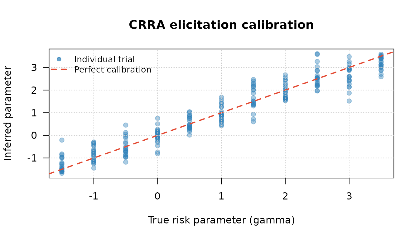
Inferred vs true risk parameter across 340 simulated sessions. Points cluster around the identity line, showing asymptotically correct recovery.
Points cluster around the identity line throughout the range, confirming the algorithm is asymptotically unbiased. The spread around the line is the residual elicitation uncertainty — exactly what the posterior in the sensitivity analysis captures.
MAE by true parameter value
mae_by_param <- aggregate(Abs_Error ~ True_Param, data = results, FUN = mean)
colnames(mae_by_param) <- c("True_gamma", "Mean_Abs_Error")
mae_by_param$Mean_Abs_Error <- round(mae_by_param$Mean_Abs_Error, 3)
knitr::kable(mae_by_param, caption = "Mean absolute error by true gamma value.")| True_gamma | Mean_Abs_Error |
|---|---|
| -1.5 | 0.291 |
| -1.0 | 0.314 |
| -0.5 | 0.356 |
| 0.0 | 0.271 |
| 0.5 | 0.247 |
| 1.0 | 0.299 |
| 1.5 | 0.459 |
| 2.0 | 0.309 |
| 2.5 | 0.356 |
| 3.0 | 0.468 |
| 3.5 | 0.308 |
barplot(mae_by_param$Mean_Abs_Error,
        names.arg = mae_by_param$True_gamma,
        col       = "#7fcdbb",
        xlab      = "True gamma",
        ylab      = "Mean absolute error",
        main      = "Elicitation accuracy by risk aversion level",
        las       = 2)
abline(h = mean(results$Abs_Error), lty = 2, col = "#e34a33", lwd = 2)
legend("topright", legend = sprintf("Global MAE = %.3f", mean(results$Abs_Error)),
       lty = 2, col = "#e34a33", lwd = 2, bty = "n")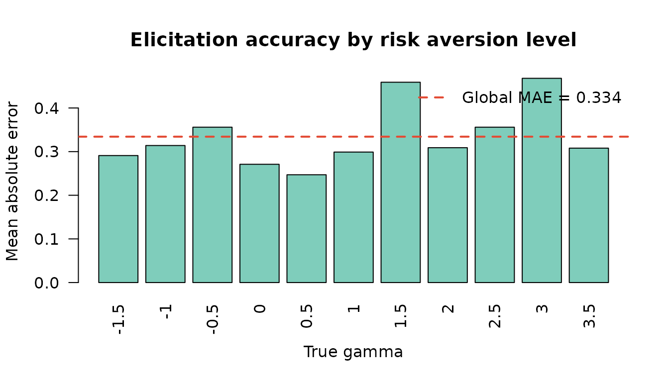
MAE across true parameter values. The dashed line is the global average.
cat("Global MAE:", round(mean(results$Abs_Error), 4), "\n")
#> Global MAE: 0.3342
cat("Fraction of trials with |error| < 0.5:",
    round(mean(results$Abs_Error < 0.5), 3), "\n")
#> Fraction of trials with |error| < 0.5: 0.75
Accuracy is best for strongly risk-averse agents (gamma > 1.5), where the utility curve is most distinctive. For most practical applications (gamma between 0.5 and 3) the inferred parameter is within 0.5 units of the truth in the majority of trials.
Connecting back to the sensitivity analysis
The robot calibration quantifies the spread visible in the sensitivity plot above: the width of the posterior in Part 2 corresponds directly to the MAE at that true gamma value. A wide posterior means the elicitation is uncertain — and the sensitivity analysis shows how much that translates into VOI uncertainty. Where the gradient is steep (Part 2 gradient plot) and MAE is large (the MAE bar chart), the credible interval on VOI will be widest.
The robot validation gives an upper bound on accuracy — real
respondents may be noisier than the simulated agent. When in doubt, the
95 % credible interval from rp$param_ci passed to
voi_sensitivity() gives a conservative range for the VOI
estimate.