8. Case Study: Fishing Location Choice (Mantyniemi et al. 2009)

Key terms used in this vignette

EVPI — the maximum any study is worth; the gain from knowing the true state before deciding. Property 2 — no action is safe in all states; every choice is wrong somewhere, so uncertainty is costly. Risk aversion (γ) — γ = 0 is risk-neutral; γ > 0 penalises bad outcomes more heavily. Certainty equivalent (CE) — the guaranteed catch a risk-averse manager considers as good as the uncertain gamble. See vira-01-concepts for full definitions.

What this vignette shows

When no action is safe (fishing the wrong location always produces a poor catch), EVPI is near its theoretical maximum.
Under risk aversion, this already-high EVPI rises further: the manager’s certainty equivalent without information falls, making perfect information even more attractive.
This is the opposite pattern from Property 1 cases (vignette 6), where risk aversion drives EVPI toward zero.

Part 1 — Two-location fishing

Background

Mäntyniemi et al. (2009) describe a fisheries decision in which a manager must choose where to fish — offshore or in an estuary — without knowing which location holds the larger share of the population. Either choice can be wrong; there is no neutral fallback. The manager has prior knowledge that the estuary holds most of the fish 70 % of the time.

Holden et al. (2024) use this case to illustrate that the symmetric utility structure (equal stakes in both directions) can produce the highest EVPI possible in any two-action, two-state problem — higher than all seven million random systems they simulated.

Decision table

A population of 1000 fish moves between two habitats. By placing gear in the right habitat, the manager catches 800 fish; in the wrong habitat, only 200. Both choices carry equal downside risk — there is no safe fallback.

Action	80 % in estuary (P = 0.7)	80 % offshore (P = 0.3)
Fish estuary	800	200
Fish offshore	200	800

Key structural feature: neither action dominates. Fishing in the estuary is right when most fish are there but wrong otherwise, and vice versa.

data("mantyniemi2009_fishing")
V       <- mantyniemi2009_fishing$V_location
p_prior <- mantyniemi2009_fishing$p_location

str(mantyniemi2009_fishing)
#> List of 4
#>  $ V_location: num [1:2, 1:2] 800 200 200 800
#>   ..- attr(*, "dimnames")=List of 2
#>   .. ..$ action: chr [1:2] "fish_estuary" "fish_offshore"
#>   .. ..$ state : chr [1:2] "most_estuary" "most_offshore"
#>  $ p_location: Named num [1:2] 0.7 0.3
#>   ..- attr(*, "names")= chr [1:2] "most_estuary" "most_offshore"
#>  $ V_herring : num [1:3, 1:2] 1235 1000 740 841 1000 ...
#>   ..- attr(*, "dimnames")=List of 2
#>   .. ..$ action: chr [1:3] "X_1.25" "X_1.50" "X_1.75"
#>   .. ..$ state : chr [1:2] "BH_true" "Ricker_true"
#>  $ p_herring : Named num [1:2] 0.43 0.57
#>   ..- attr(*, "names")= chr [1:2] "BH_true" "Ricker_true"

Risk-neutral EVPI

Without information, the manager fishes the estuary (the more likely location). This pipeline computes how much better the manager would do with perfect information.

problem <- voi_problem(V, p_prior)

result_rn <- problem |>
  transform_to_utility() |>
  optimize_action() |>
  calculate_utility_dist() |>
  summarize_utility() |>
  transform_to_values() |>
  calculate_value_info()

cat("Expected catch without information: ", result_rn$EV_uncertainty, "fish\n")
#> Expected catch without information:  620 fish
cat("Expected catch with perfect info:   ", result_rn$EV_certainty,   "fish\n")
#> Expected catch with perfect info:    800 fish
cat("EVPI (risk-neutral):                ", round(result_rn$value_info, 2), "fish\n")
#> EVPI (risk-neutral):                 180 fish

The EVPI is 180 fish, meaning a study that perfectly reveals fish location before the decision is worth up to 180 fish. This is large because:

The stakes are high: fishing the wrong location costs 600 fish (800 − 200).
There is no safe action: every choice is wrong 30 % of the time.
The prior is not too far from 50/50, so the “wrong choice” risk is material.

How close to the theoretical maximum? The highest possible EVPI for this utility structure — when the prior is exactly 50/50 — would be 300 fish (half the 600-fish stake). Because the prior here is 70/30, the actual EVPI (180 fish) is 60 % of that maximum. Holden et al. (2024) show this 300-fish ceiling is higher than all seven million random two-action, two-state systems they simulated.

stake <- max(V) - min(V)  # the cost of choosing the wrong location
cat("Stake (cost of wrong choice): ", stake, "fish\n")
#> Stake (cost of wrong choice):  600 fish
cat("EVPI:                         ", round(result_rn$value_info, 1), "fish\n")
#> EVPI:                          180 fish
cat("EVPI as % of stake:           ", round(result_rn$value_info / stake * 100, 1), "%\n")
#> EVPI as % of stake:            30 %
cat("Max possible EVPI (at 50/50): ", 0.5 * stake, "fish\n")
#> Max possible EVPI (at 50/50):  300 fish

Risk-averse EVPI

A risk-averse manager dislikes the 30 % chance of catching only 200 fish more than they enjoy the 70 % chance of catching 800. Their certainty equivalent — the guaranteed catch they consider equally attractive to the gamble — is below the expected value of 620 fish.

Because there is no safe action to retreat to, risk aversion makes the gamble feel worse without providing an escape route. Perfect information eliminates the gamble entirely (the manager always fishes the right location), so it becomes even more valuable.

# Set up risk-averse preferences: CRRA with gamma = 1 (moderate risk aversion)
rp  <- risk_preference("CRRA", param = 1, val_min = 0, val_max = 1000,
                       outcome_name = "fish", maximize = TRUE)
fns <- use_risk_preference(rp)

# Same six-step pipeline, but with risk-averse utility transformation
result_ra <- problem |>
  transform_to_utility(fns$utility) |>
  optimize_action() |>
  calculate_utility_dist() |>
  summarize_utility() |>
  transform_to_values(fns$inv_utility) |>
  calculate_value_info()

cat("Certainty equivalent without information: ", round(result_ra$EV_uncertainty, 1), "fish\n")
#> Certainty equivalent without information:  527.8 fish
cat("Certainty equivalent with perfect info:   ", round(result_ra$EV_certainty,   1), "fish\n")
#> Certainty equivalent with perfect info:    800 fish
cat("EVPI (risk-averse, gamma = 1):            ", round(result_ra$value_info,     1), "fish\n")
#> EVPI (risk-averse, gamma = 1):             272.2 fish

cat("EVPI comparison\n")
#> EVPI comparison
cat("  Risk-neutral (gamma = 0): ", round(result_rn$value_info, 1), "fish\n")
#>   Risk-neutral (gamma = 0):  180 fish
cat("  Risk-averse  (gamma = 1): ", round(result_ra$value_info, 1), "fish\n")
#>   Risk-averse  (gamma = 1):  272.2 fish
cat("  Ratio (RA/RN):            ", round(result_ra$value_info / result_rn$value_info, 2), "\n")
#>   Ratio (RA/RN):             1.51

How EVPI responds as risk aversion increases

The plot below sweeps γ from risk-seeking (γ < 0) through risk-neutral (γ = 0) to strongly risk-averse (γ = 4). The EVPI rises monotonically — the more the manager dislikes a bad catch, the more they value knowing where the fish are.

sens <- voi_sensitivity(problem, rp, param_grid = seq(-1, 4, by = 0.1))

plot(sens$param, sens$voi,
     type = "l", lwd = 2, col = "#e34a33",
     xlab = "Risk aversion (gamma; 0 = risk-neutral, higher = more averse)",
     ylab = "EVPI (certainty equivalent, fish)",
     main = "Fishing location: EVPI rises with risk aversion",
     ylim = c(0, max(sens$voi, na.rm = TRUE) * 1.1))
abline(v = 0,       lty = 2, col = "grey50")
abline(h = result_rn$value_info, lty = 3, col = "grey50")
legend("topleft",
       legend = c("EVPI curve",
                  "Risk-neutral (gamma = 0)",
                  sprintf("Risk-neutral EVPI = %.0f fish", result_rn$value_info)),
       lty = c(1, 2, 3), col = c("#e34a33", "grey50", "grey50"),
       lwd = c(2, 1, 1), bty = "n")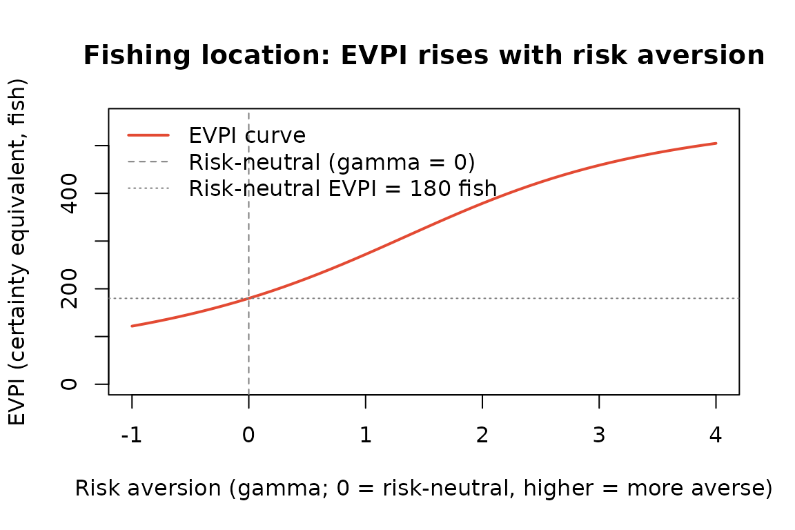

EVPI rises monotonically with risk aversion when no safe fallback exists (Property 2). Dashed lines mark the risk-neutral benchmark.

Contrast with Property 1: in the Runge whooping crane case (vignette 4), “restore meadows” is the best action under every hypothesis — a dominant safe choice. A risk-averse crane manager locks onto this safe choice even more firmly, so EVPI stays at zero. See vignette 4 for that mirror-image result.

Part 2 — North Sea Herring: Structural Model Uncertainty

Background

The second example in Mäntyniemi et al. (2009) applies value of information to uncertainty about which ecological model is correct for North Sea herring (Clupea harengus). Rather than choosing where to fish, the manager must choose how hard to fish — and the right fishing level depends on which population model is true.

This is a different flavour of Property 2: both models could be correct, and the optimal fishing strategy under one model is a poor choice under the other.

The structural uncertainty

A Bayesian population model was fitted to catch and survey data from 1960–2003 under two competing hypotheses about how herring recruitment responds to stock size:

Model	Ecological meaning	Posterior probability
Beverton-Holt	Density-compensatory recruitment (stock recovers well at low numbers)	P = 0.43
Ricker	Overcompensatory recruitment (stock can collapse at moderate fishing)	P = 0.57

The management decision is a fishing multiplier X applied to the 2003 fishing rate, projected 20 years forward. Utility is discounted profit in million NOK (Norwegian kroner).

Knowledge state	Best fishing multiplier	Why
Current uncertainty (both models)	X = 1.5	Compromise across the two models
Beverton-Holt confirmed true	X = 1.25	Lower fishing is optimal (conservative stock)
Ricker confirmed true	X = 1.75	Higher fishing is optimal (more resilient stock)

The uncertainty-optimal X = 1.5 is not just an average; it is the point of highest expected profit across all possible X values given the uncertainty.

VOI calculation

The value of information equals the expected improvement from switching away from the uncertainty-optimal X = 1.5 once uncertainty is resolved. For each model, there is a gain from adopting the model-specific best strategy instead of X = 1.5:

Gain if Beverton-Holt confirmed: switch from X = 1.5 to X = 1.25 → +235 million NOK
Gain if Ricker confirmed: switch from X = 1.5 to X = 1.75 → +243 million NOK

p_BH <- 0.43
p_R  <- 1 - p_BH
gain_BH <- 235   # million NOK gained by switching to X=1.25 when BH is true
gain_R  <- 243   # million NOK gained by switching to X=1.75 when Ricker is true

VoI_herring <- p_BH * gain_BH + p_R * gain_R
cat("VOI = P(BH) × gain(BH) + P(Ricker) × gain(Ricker)\n")
#> VOI = P(BH) × gain(BH) + P(Ricker) × gain(Ricker)
cat("    = ", p_BH, "×", gain_BH, "+", p_R, "×", gain_R, "\n")
#>     =  0.43 × 235 + 0.57 × 243
cat("    = ", round(VoI_herring), "million NOK\n")
#>     =  240 million NOK

The result matches the paper: VoI ≈ 240 million NOK. This is the maximum price the agency should pay for research that perfectly identifies the true model before the next management cycle.

The cost of overconfidence

What if a manager ignores the uncertainty and acts as if one model is definitely correct? The paper also computes these “overconfidence losses”:

Assume Beverton-Holt is true and fish at X = 1.25, but Ricker is actually true: −159 million NOK
Assume Ricker is true and fish at X = 1.75, but Beverton-Holt is actually true: −260 million NOK

loss_assume_BH_wrong  <- -159  # overfished under Ricker
loss_assume_R_wrong   <- -260  # underfished under Beverton-Holt

cat("Loss if assume BH correct but Ricker is true:   ",
    loss_assume_BH_wrong, "million NOK\n")
#> Loss if assume BH correct but Ricker is true:    -159 million NOK
cat("Loss if assume Ricker correct but BH is true:   ",
    loss_assume_R_wrong,  "million NOK\n")
#> Loss if assume Ricker correct but BH is true:    -260 million NOK
cat("\nIf forced to guess, assuming Beverton-Holt is the safer overconfidence\n")
#> 
#> If forced to guess, assuming Beverton-Holt is the safer overconfidence
cat("(expected loss 90 million NOK less than assuming Ricker).\n")
#> (expected loss 90 million NOK less than assuming Ricker).

The Ricker overconfidence is more dangerous. If a manager must ignore uncertainty, assuming Beverton-Holt and fishing conservatively at X = 1.25 is the less risky gamble.

Approximating the herring problem in vira

The herring problem uses a continuous fishing-level variable (X can be any value), but vira works with a fixed set of discrete actions. We approximate it using the three representative fishing levels from the paper, with utility values anchored to a common baseline.

Why the vira number differs from the paper: The paper’s VOI (240 million NOK) is computed relative to the uncertainty-optimal X = 1.5, which is the peak of a continuous curve across all possible X. In the discrete three-action version, X = 1.75 happens to score slightly higher than X = 1.5 — shifting the “no-information baseline” and reducing the computed EVPI to ~213 million NOK. The difference (≈27 million NOK) represents information already embedded in the discrete choice of X = 1.75 that is invisible in the continuous setting. Both numbers are correct for their respective framings.

V_herring <- mantyniemi2009_fishing$V_herring
p_herring <- mantyniemi2009_fishing$p_herring
print(V_herring)
#>         state
#> action   BH_true Ricker_true
#>   X_1.25    1235         841
#>   X_1.50    1000        1000
#>   X_1.75     740        1243

problem_herring <- voi_problem(V_herring, p_herring)

result_herring_rn <- problem_herring |>
  transform_to_utility() |>
  optimize_action() |>
  calculate_utility_dist() |>
  summarize_utility() |>
  transform_to_values() |>
  calculate_value_info()

cat("EV without info (discrete best action): ",
    round(result_herring_rn$EV_uncertainty, 1), "million NOK\n")
#> EV without info (discrete best action):  1026.7 million NOK
cat("EV with perfect information:            ",
    round(result_herring_rn$EV_certainty,   1), "million NOK\n")
#> EV with perfect information:             1239.6 million NOK
cat("EVPI (discrete 3-action approx.):       ",
    round(result_herring_rn$value_info,     1), "million NOK\n")
#> EVPI (discrete 3-action approx.):        212.8 million NOK
cat("VOI  (paper, continuous baseline):      ",
    round(VoI_herring),                         "million NOK\n")
#> VOI  (paper, continuous baseline):       240 million NOK

Risk-averse extension

Under risk aversion, the upside gains (fishing with the right model) are weighted less heavily while the downside losses (fishing with the wrong model) are penalised more. Because the Ricker-optimal strategy (X = 1.75) has a much larger downside under Beverton-Holt (−260) than the Beverton-Holt-optimal strategy has under Ricker (−159), a risk-averse manager shifts away from X = 1.75 as γ increases.

rp_herring  <- risk_preference("CRRA", param = 1, val_min = 500, val_max = 1500,
                                outcome_name = "million NOK", maximize = TRUE)
fns_herring <- use_risk_preference(rp_herring)

result_herring_ra <- problem_herring |>
  transform_to_utility(fns_herring$utility) |>
  optimize_action() |>
  calculate_utility_dist() |>
  summarize_utility() |>
  transform_to_values(fns_herring$inv_utility) |>
  calculate_value_info()

cat("EVPI (risk-neutral, gamma = 0): ",
    round(result_herring_rn$value_info, 1), "million NOK\n")
#> EVPI (risk-neutral, gamma = 0):  212.8 million NOK
cat("EVPI (risk-averse,  gamma = 1): ",
    round(result_herring_ra$value_info, 1), "million NOK\n")
#> EVPI (risk-averse,  gamma = 1):  239.5 million NOK

sens_herring <- voi_sensitivity(problem_herring, rp_herring,
                                param_grid = seq(-1, 3, by = 0.1))

plot(sens_herring$param, sens_herring$voi,
     type = "l", lwd = 2, col = "#2c7fb8",
     xlab = "Risk aversion (gamma; 0 = risk-neutral, higher = more averse)",
     ylab = "EVPI (million NOK, discrete approx.)",
     main = "North Sea herring: EVPI vs risk aversion",
     ylim = c(0, max(sens_herring$voi, na.rm = TRUE) * 1.1))
abline(v = 0, lty = 2, col = "grey50")
abline(h = result_herring_rn$value_info, lty = 3, col = "grey50")
legend("topleft",
       legend = c("EVPI curve",
                  sprintf("Risk-neutral EVPI ≈ %.0f M NOK",
                          result_herring_rn$value_info)),
       lty = c(1, 3), col = c("#2c7fb8", "grey50"), lwd = 2, bty = "n")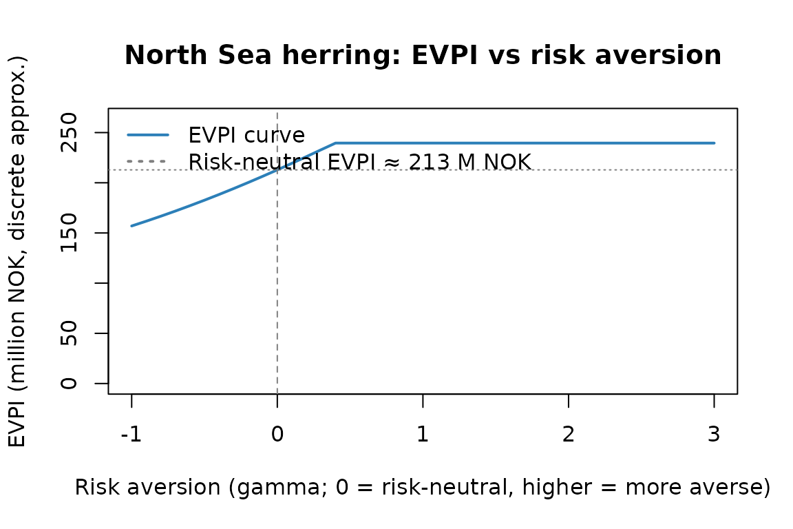

EVPI for the North Sea herring structural-model problem as a function of risk aversion (discrete 3-action approximation). The non-monotone shape reflects the asymmetric downside risks across models.

Unlike the symmetric fishing-location problem (Part 1), the herring EVPI does not rise monotonically with risk aversion. The asymmetry between models — the Ricker downside is much worse than the Beverton-Holt downside — means the manager’s optimal action shifts as γ increases, changing which states drive EVPI.

References

Mäntyniemi, S., Kuikka, S., Rahikainen, M., Kell, L.T. & Kaitala, V. (2009). The value of information in fisheries management: North Sea herring as an example. ICES Journal of Marine Science, 66, 2278–2283.

Holden, M.H., Akinlotan, M., Binley, A.D., Cho, F., Helmstedt, K.J. & Chadès, I. (2024). Why shouldn’t I collect more data? Reconciling disagreements between intuition and value of information analyses. Methods in Ecology and Evolution, 15, 1580–1592. DOI: 10.1111/2041-210X.14391

Property 2 — No safe action exists; EVPI is near-maximum and rises with risk aversion

Key terms used in this vignette

What this vignette shows

Part 1 — Two-location fishing

Background

Decision table

Risk-neutral EVPI

Risk-averse EVPI

How EVPI responds as risk aversion increases

Part 2 — North Sea Herring: Structural Model Uncertainty

Background

The structural uncertainty

VOI calculation

The cost of overconfidence

Approximating the herring problem in vira

Risk-averse extension

References