4. Expected Value of Partial Perfect Information (EVPXI) • vira

EVPXI: the value of resolving one uncertainty at a time

EVPXI — the Expected Value of Partial Perfect Information — measures how much management performance would improve if one specific uncertainty were resolved perfectly while all others remained unknown. It is calculated separately for each candidate uncertainty, producing a ranking of which uncertainties most impede the decision.

Specifically, let the outcomes of the partial information source for state $i$ be $k \in \{\text{confirmed}, \text{refuted}\}$ . The probability of each outcome is:

$pp_{\text{confirmed}} = p[i]$
$pp_{\text{refuted}} = 1 - p[i]$

For each outcome $k$ , the posterior probability vector $\mathbf{p}_k$ is:

If confirmed: $p_{\text{confirmed}}[s] = 1$ if $s = i$ , and $0$ otherwise.
If refuted: $p_{\text{refuted}}[s] = 0$ if $s = i$ , and $p[s] / (1 - p[i])$ if $s \neq i$ .

The EVPXI is calculated by comparing the expected utility with this partial information to the expected utility under the prior:

$\mathrm{EVPXI}(i) = \mathrm{EU}_{\text{cert}} - \mathrm{EU}_{\text{unc}}$

where:

$\mathrm{EU}_{\text{cert}} = \sum_k pp_k \max_a \sum_s U[a, s] \cdot p_k[s]$ $\mathrm{EU}_{\text{unc}} = \max_a \sum_s U[a, s] \cdot p[s]$

A key practical point: when testing an individual hypothesis perfectly, there are only two outcomes — confirmed (posterior weight = 1 on that state, 0 elsewhere) or refuted (weight = 0 on that state, all remaining hypotheses rescaled in proportion to their original weights).

Case study: Eastern Migratory Population of whooping cranes

Runge, Converse & Lyons (2011) applied EVPXI to management of the Eastern Migratory Population (EMP) of whooping cranes (Grus americana) at Necedah National Wildlife Refuge (NNWR). Birds had near-zero reproductive success through 2009 despite acceptable survival rates. Eight competing hypotheses about the cause of reproductive failure were evaluated against seven management strategies, scored on a composite 0–1 scale across four weighted objectives (number of pairs, fledging rate, adult survival, body condition on departure).

Decision table (composite weighted score, Table 5 of Runge et al. 2011)

data("runge2011_crane")
V_crane <- runge2011_crane$V
p_crane <- runge2011_crane$p

Step 1: Verify EVPI = 0.117

The paper reports EVPI = 0.117 on the composite 0–1 scale (performance rises from 0.590 to 0.707, a 19.9% gain). We reproduce this first.

result_evpi <- suppressMessages(
  voi_problem(V_crane, p_crane) |>
    transform_to_utility() |>
    optimize_action() |>
    calculate_utility_dist() |>
    summarize_utility() |>
    transform_to_values() |>
    calculate_value_info()
)

cat("Best action (no info):       ", rownames(V_crane)[result_evpi$a_uncertainty[1]], "\n")
#> Best action (no info):        restore_meadows
cat("EV without information:      ", round(result_evpi$EV_uncertainty, 3),
    " (published: 0.590)\n")
#> EV without information:       0.59  (published: 0.590)
cat("EV with perfect information: ", round(result_evpi$EV_certainty, 3),
    " (published: 0.707)\n")
#> EV with perfect information:  0.707  (published: 0.707)
cat("EVPI:                        ", round(result_evpi$value_info, 3),
    " (published: 0.117)\n")
#> EVPI:                         0.117  (published: 0.117)

Step 2: EVPXI for each hypothesis

For each hypothesis $i$ we construct a two-outcome posterior:

Confirmed (probability = $p_i$ ): posterior concentrates weight 1 on state $i$ , zero elsewhere.
Refuted (probability = $1 - p_i$ ): posterior places weight 0 on state $i$ and rescales all remaining hypothesis weights proportionally.

# Helper: EVPXI for hypothesis index i (1-indexed), optionally with risk preference
evpxi_for_hypothesis <- function(V, p, i, rp = NULL) {
  S <- length(p)

  post_confirmed        <- numeric(S)
  post_confirmed[i]     <- 1

  post_refuted          <- p
  post_refuted[i]       <- 0
  post_refuted          <- post_refuted / sum(post_refuted)

  p_post    <- matrix(c(post_confirmed, post_refuted), nrow = 2, byrow = TRUE)
  p_outcome <- c(p[i], 1 - p[i])

  prob <- voi_problem(V, p, p_post, p_outcome)
  if (!is.null(rp)) {
    fns <- use_risk_preference(rp)
    result <- suppressMessages(
      prob |>
        transform_to_utility(fns$utility) |>
        optimize_action() |>
        calculate_utility_dist() |>
        summarize_utility() |>
        transform_to_values(fns$inv_utility) |>
        calculate_value_info()
    )
  } else {
    result <- suppressMessages(
      prob |>
        transform_to_utility() |>
        optimize_action() |>
        calculate_utility_dist() |>
        summarize_utility() |>
        transform_to_values() |>
        calculate_value_info()
    )
  }
  result$value_info
}

S <- ncol(V_crane)
evpxi_vals <- setNames(
  vapply(seq_len(S), function(i) evpxi_for_hypothesis(V_crane, p_crane, i),
         numeric(1)),
  colnames(V_crane)
)

# Summary table
evpxi_df <- data.frame(
  hypothesis    = names(evpxi_vals),
  prior_weight  = round(p_crane * 100, 1),
  EVPXI         = round(evpxi_vals, 4),
  pct_of_EVPI   = round(evpxi_vals / result_evpi$value_info * 100, 1),
  stringsAsFactors = FALSE
)
evpxi_df[order(-evpxi_df$EVPXI), ]
#>                              hypothesis prior_weight  EVPXI pct_of_EVPI
#> black_flies                 black_flies         29.1 0.0628        53.6
#> disturbance                 disturbance         10.0 0.0377        32.2
#> egg_salvage                 egg_salvage          4.4 0.0099         8.5
#> social_conditioning social_conditioning         11.9 0.0067         5.7
#> too_young                     too_young          9.4 0.0000         0.0
#> nutr_nnwr                     nutr_nnwr         22.8 0.0000         0.0
#> nutr_winter                 nutr_winter          5.9 0.0000         0.0
#> nutr_both                     nutr_both          6.6 0.0000         0.0

The partial EVPXIs match the published values:

Hypothesis	Published share	Computed share
Black flies (H2)	54%	~54%
Human disturbance (H8)	32%	~32%
Egg salvage (H7)	8%	~8%
Social conditioning (H3)	6%	~6%
All others	< 1% each	< 1% each

Step 3: Do the partial EVPXIs add up to EVPI?

Runge et al. note: “as it turns out in this case, the partial EVPIs do sum to the total EVPI” (Fig. 2). We verify:

cat("Sum of all EVPXI:  ", round(sum(evpxi_vals), 4), "\n")
#> Sum of all EVPXI:   0.117
cat("Total EVPI:        ", round(result_evpi$value_info, 4), "\n")
#> Total EVPI:         0.117
cat("Difference:        ", round(sum(evpxi_vals) - result_evpi$value_info, 6), "\n")
#> Difference:         0

This additive property is not guaranteed in general (the EVPXI formula explicitly warns against it), but it holds here because the switching hypotheses are nearly independent in how they drive action changes.

Step 4: Visualise the EVPXI profile

evpxi_ordered <- sort(evpxi_vals, decreasing = TRUE)
hyp_labels <- c(
  too_young           = "Too young",
  black_flies         = "Black flies",
  social_conditioning = "Social cond.",
  nutr_nnwr           = "Nutr. (NNWR)",
  nutr_winter          = "Nutr. (winter)",
  nutr_both            = "Nutr. (both)",
  egg_salvage          = "Egg salvage",
  disturbance         = "Disturbance"
)

cols <- ifelse(evpxi_vals[names(evpxi_ordered)] > 0.005,
               "#2c7fb8", "#bdbdbd")

mp <- barplot(
  evpxi_ordered,
  names.arg = hyp_labels[names(evpxi_ordered)],
  col   = cols,
  ylab  = "EVPXI (composite score units)",
  main  = "Partial EVPI per hypothesis — Runge et al. (2011)",
  las   = 2,
  cex.names = 0.8,
  ylim  = c(0, max(evpxi_ordered) * 1.25)
)
abline(h = result_evpi$value_info, lty = 2, col = "grey40")
text(x = max(mp) * 0.7, y = result_evpi$value_info * 1.05,
     labels = sprintf("Total EVPI = %.3f", result_evpi$value_info),
     col = "grey40", cex = 0.85)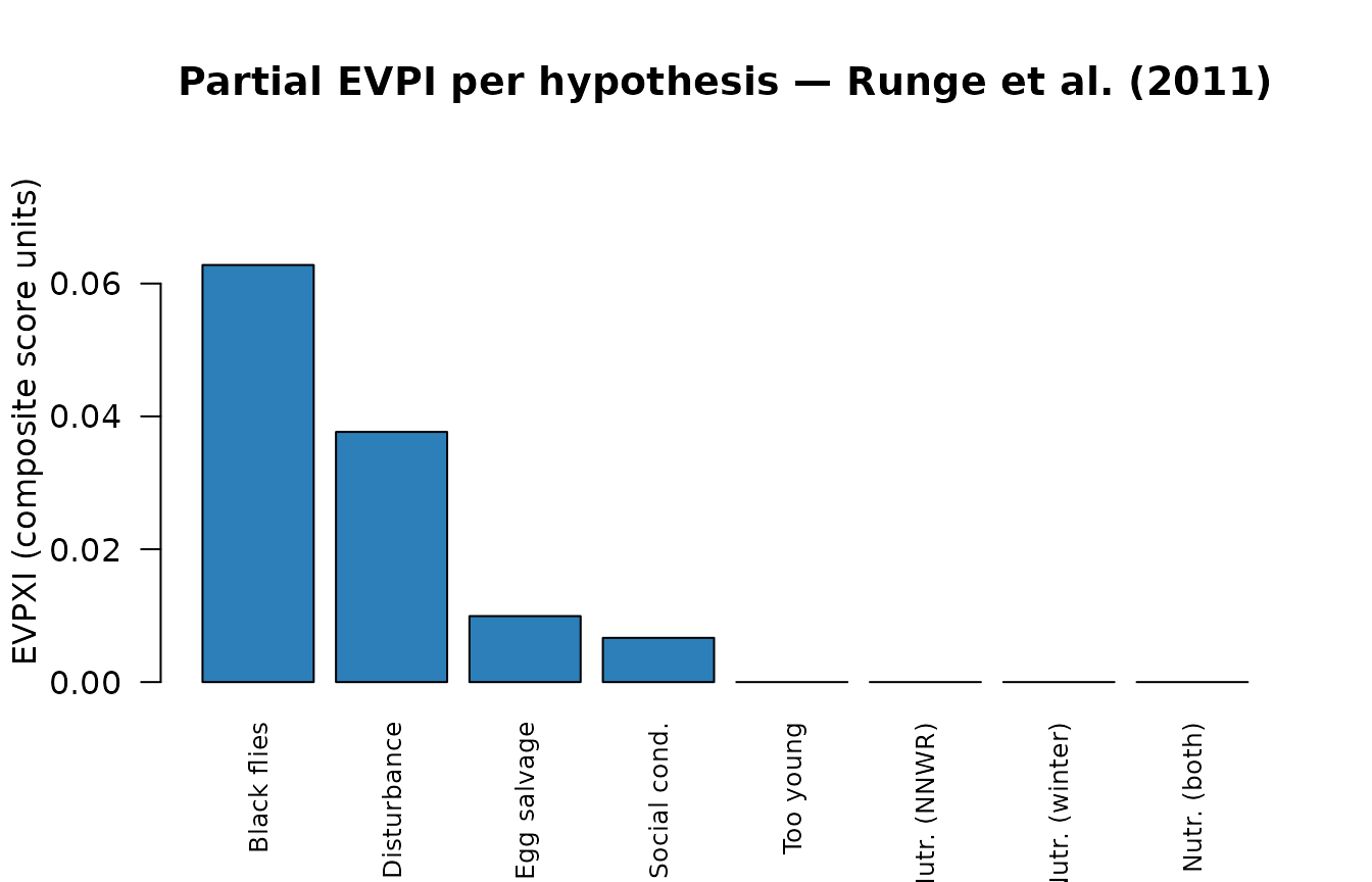

The black-fly and human-disturbance hypotheses together account for 86% of the total information value, guiding where monitoring effort should focus.

Step 5: EVPXI under risk aversion

Under risk aversion, the decision-maker dislikes variance and penalizes bad outcomes. We can model this by defining a Constant Relative Risk Aversion (CRRA) utility function. Since the composite scores range between 0 and 1, we set val_min = 0 and val_max = 1.

Here we calculate the EVPXI for each hypothesis under different levels of risk aversion ( $\gamma = 1$ representing log utility, and $\gamma = 2$ representing stronger risk aversion):

# Define risk preferences
rp_gamma1 <- risk_preference("CRRA", param = 1, val_min = 0, val_max = 1,
                             outcome_name = "composite score", maximize = TRUE)
rp_gamma2 <- risk_preference("CRRA", param = 2, val_min = 0, val_max = 1,
                             outcome_name = "composite score", maximize = TRUE)

# Calculate EVPXI for all hypotheses
evpxi_rn   <- evpxi_vals
evpxi_ra1  <- setNames(
  vapply(seq_len(S), function(i) evpxi_for_hypothesis(V_crane, p_crane, i, rp_gamma1), numeric(1)),
  colnames(V_crane)
)
evpxi_ra2  <- setNames(
  vapply(seq_len(S), function(i) evpxi_for_hypothesis(V_crane, p_crane, i, rp_gamma2), numeric(1)),
  colnames(V_crane)
)

# Compare in a table
evpxi_comparison <- data.frame(
  hypothesis   = hyp_labels[names(evpxi_vals)],
  risk_neutral = round(evpxi_rn, 4),
  gamma_1      = round(evpxi_ra1, 4),
  gamma_2      = round(evpxi_ra2, 4),
  stringsAsFactors = FALSE
)
evpxi_comparison[order(-evpxi_comparison$risk_neutral), ]
#>                         hypothesis risk_neutral gamma_1 gamma_2
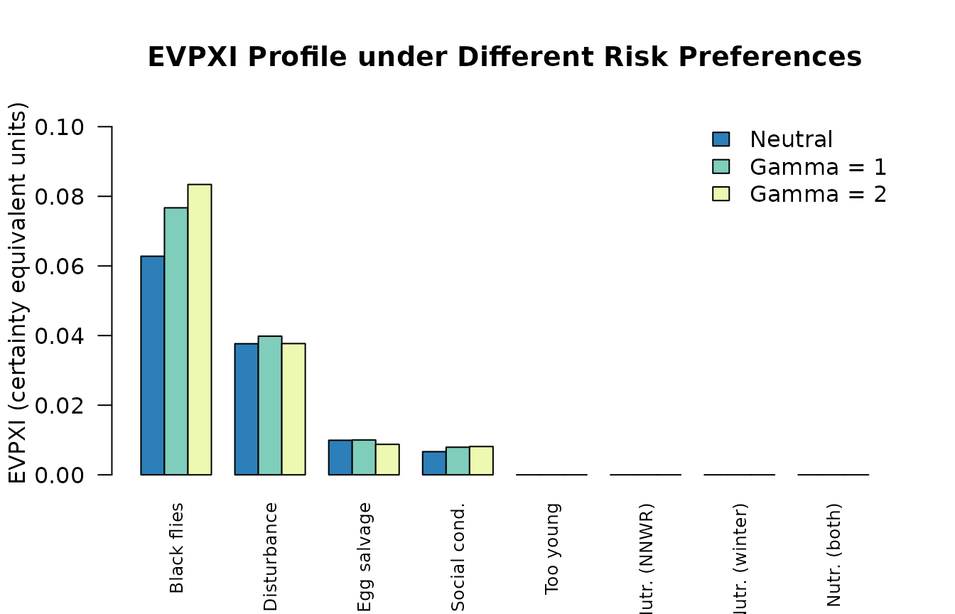
#> black_flies            Black flies       0.0628  0.0767  0.0834
#> disturbance            Disturbance       0.0377  0.0398  0.0377
#> egg_salvage            Egg salvage       0.0099  0.0100  0.0088
#> social_conditioning   Social cond.       0.0067  0.0079  0.0081
#> too_young                Too young       0.0000  0.0000  0.0000
#> nutr_nnwr             Nutr. (NNWR)       0.0000  0.0000  0.0000
#> nutr_winter         Nutr. (winter)       0.0000  0.0000  0.0000
#> nutr_both             Nutr. (both)       0.0000  0.0000  0.0000

As risk aversion increases: * The value of resolving the critical uncertainty (Black flies) increases from 0.0628 (risk-neutral) to 0.0767 ( $\gamma = 1$ ) and 0.0834 ( $\gamma = 2$ ). * Similarly, resolving the Human disturbance uncertainty is valued at 0.0377 under risk neutrality, rising to 0.0398 ( $\gamma = 1$ ) before slightly decreasing to 0.0377 ( $\gamma = 2$ ). * The sum of individual EVPXIs also increases overall under risk aversion, reflecting how a risk-averse manager is more willing to invest in resolving uncertainties to avoid low-utility, high-variance outcomes.

We can visualize how the partial information profiles change across these three risk settings:

# Group data for barplot
plot_data <- rbind(
  Neutral = evpxi_rn,
  "Gamma = 1" = evpxi_ra1,
  "Gamma = 2" = evpxi_ra2
)
colnames(plot_data) <- hyp_labels[colnames(plot_data)]

# Re-order by risk-neutral value
ordered_cols <- order(-evpxi_rn)
plot_data <- plot_data[, ordered_cols]

barplot(
  plot_data,
  beside = TRUE,
  col = c("#2c7fb8", "#7fcdbb", "#edf8b1"),
  legend.text = TRUE,
  args.legend = list(x = "topright", bty = "n"),
  ylab = "EVPXI (certainty equivalent units)",
  main = "EVPXI Profile under Different Risk Preferences",
  las = 2,
  cex.names = 0.8,
  ylim = c(0, max(plot_data) * 1.25)
)

Interpretation

The two practically informative hypotheses drive fundamentally different management responses:

Black flies → best action is No salvage (0.589), not the naive “kill flies” strategy
Human disturbance → best action is Swap eggs (0.740)

All other hypotheses favour Restore meadows, which is also the best action under the prior. Resolving them would not change the management recommendation. This is the defining condition for low EVPXI: information has value only when it could change what you decide to do.

References

Runge, M.C., Converse, S.J. & Lyons, J.E. (2011). Which uncertainty? Using expert elicitation and expected value of information to design an adaptive program. Biological Conservation, 144, 1214–1223. DOI: 10.1016/j.biocon.2010.12.020

Yokota, F. & Thompson, K.M. (2004). Value of information literature analysis: a review of applications in health risk management. Medical Decision Making, 24, 287–298.