6. Case Study: Species Protection (Bennett et al. 2018)

Key terms used in this vignette

EVPI — the maximum any study is worth; the gain from knowing the true state before deciding. EVSI — like EVPI but for an imperfect, real-world survey. Property 1 — one action is best in all states; information cannot change the decision, so EVPI = 0. Property 2 — no action is safe in all states; uncertainty is costly and EVPI > 0. Risk aversion (γ) — γ = 0 is risk-neutral; γ > 0 penalises bad outcomes more heavily. See vira-01-concepts for full definitions.

What this vignette shows

For a single parcel or single species with unlimited budget, the “protect/manage” action is dominant — monitoring before acting provides zero benefit (EVPI = 0).
This flips completely once the manager has many units but a limited budget: the budget forces a prioritisation decision, the dominant action disappears, and monitoring now has positive value.
For a multi-species scenario, an additional complication arises: monitoring carries an extinction risk during the delay. Under risk aversion, that extinction risk looms larger and can erode the case for monitoring.
Whether monitoring is worthwhile depends not just on the biology but on the decision structure — specifically, whether a budget forces trade-offs between units.

Part 1 — Single parcel: protecting always wins

Background

Bennett et al. (2018) develop a multi-unit VOI framework for conservation planning. Their Case Study 1 concerns a manager deciding whether to protect parcels that may or may not harbour a focal threatened species.

The key result is a reversal: monitoring has zero value per parcel but positive value across a portfolio of parcels under a binding budget. This section works through both situations.

Decision table

Action	Species present	Species absent
Protect	1	0
Do not protect	0	0

Protecting produces a benefit of 1 when the species is there and 0 when it is not. Not protecting always produces 0 — there is no harm from protecting an empty site, but there is also no benefit.

“Protect” weakly dominates: it is strictly better when the species is present and exactly equal when it is absent. No monitoring result can make “do not protect” the better choice.

data("bennett2018_parcel")
V_parcel <- bennett2018_parcel$V_parcel
p_high   <- bennett2018_parcel$p_high
p_low    <- bennett2018_parcel$p_low
str(bennett2018_parcel)
#> List of 5
#>  $ V_parcel: num [1:2, 1:2] 1 0 0 0
#>   ..- attr(*, "dimnames")=List of 2
#>   .. ..$ action: chr [1:2] "protect" "do_not_protect"
#>   .. ..$ state : chr [1:2] "present" "absent"
#>  $ p_high  : Named num [1:2] 0.5 0.5
#>   ..- attr(*, "names")= chr [1:2] "present" "absent"
#>  $ p_low   : Named num [1:2] 0.1 0.9
#>   ..- attr(*, "names")= chr [1:2] "present" "absent"
#>  $ V_budget: num [1:2, 1:4] 1 1 1 0 0 1 0 0
#>   ..- attr(*, "dimnames")=List of 2
#>   .. ..$ : chr [1:2] "protect_H" "protect_L"
#>   .. ..$ : chr [1:4] "both" "H_only" "L_only" "neither"
#>  $ p_joint : Named num [1:4] 0.05 0.45 0.05 0.45
#>   ..- attr(*, "names")= chr [1:4] "both" "H_only" "L_only" "neither"

EVPI is zero for any prior

The prior probability of the species being present does not matter — “protect” wins whenever the species could be there. The two scenarios below confirm EVPI = 0 regardless of how likely the species is.

# High-prior parcel: species present 50% of the time
problem_high <- voi_problem(V_parcel, p_high)

result_high_rn <- problem_high |>
  transform_to_utility() |>
  optimize_action() |>
  calculate_utility_dist() |>
  summarize_utility() |>
  transform_to_values() |>
  calculate_value_info()

cat("Prior P(present) = 0.5\n")
#> Prior P(present) = 0.5
cat("  EV without info:", result_high_rn$EV_uncertainty, "\n")
#>   EV without info: 0.5
cat("  EV with info:   ", result_high_rn$EV_certainty,   "\n")
#>   EV with info:    0.5
cat("  EVPI:           ", result_high_rn$value_info,      "\n")
#>   EVPI:            0

# Low-prior parcel: species present only 10% of the time
problem_low <- voi_problem(V_parcel, p_low)

result_low_rn <- problem_low |>
  transform_to_utility() |>
  optimize_action() |>
  calculate_utility_dist() |>
  summarize_utility() |>
  transform_to_values() |>
  calculate_value_info()

cat("Prior P(present) = 0.1\n")
#> Prior P(present) = 0.1
cat("  EV without info:", result_low_rn$EV_uncertainty, "\n")
#>   EV without info: 0.1
cat("  EV with info:   ", result_low_rn$EV_certainty,   "\n")
#>   EV with info:    0.1
cat("  EVPI:           ", result_low_rn$value_info,      "\n")
#>   EVPI:            0

EVPI = 0 for both priors. The dominant “protect” action means prior uncertainty is irrelevant to the information-value calculation.

EVPI is also zero under risk aversion

Under any degree of risk aversion, the optimal action remains “protect” — it weakly dominates in every state. A risk-averse manager locks onto the safe choice even more firmly.

rp <- risk_preference("CRRA", param = 1, val_min = 0, val_max = 1,
                       outcome_name = "occurrences saved", maximize = TRUE)
fns <- use_risk_preference(rp)

result_high_ra <- problem_high |>
  transform_to_utility(fns$utility) |>
  optimize_action() |>
  calculate_utility_dist() |>
  summarize_utility() |>
  transform_to_values(fns$inv_utility) |>
  calculate_value_info()

cat("P(present) = 0.5\n")
#> P(present) = 0.5
cat("  EVPI (risk-neutral):         ", result_high_rn$value_info, "\n")
#>   EVPI (risk-neutral):          0
cat("  EVPI (risk-averse, gamma=1): ", round(result_high_ra$value_info, 6), "\n")
#>   EVPI (risk-averse, gamma=1):  0

sens_high <- voi_sensitivity(problem_high, rp, param_grid = seq(-1, 4, by = 0.2))

plot(sens_high$param, sens_high$voi,
     type = "l", lwd = 2, col = "#2c7fb8",
     xlab = "Risk aversion (gamma; 0 = risk-neutral, higher = more averse)",
     ylab = "EVPI (occurrences saved)",
     main = "Single parcel: monitoring has no value\n(Property 1 — dominant action)",
     ylim = c(-0.01, 0.1))
abline(h = 0, lty = 2, col = "grey60")
legend("topright", legend = "EVPI = 0 always", lty = 2, col = "grey60", bty = "n")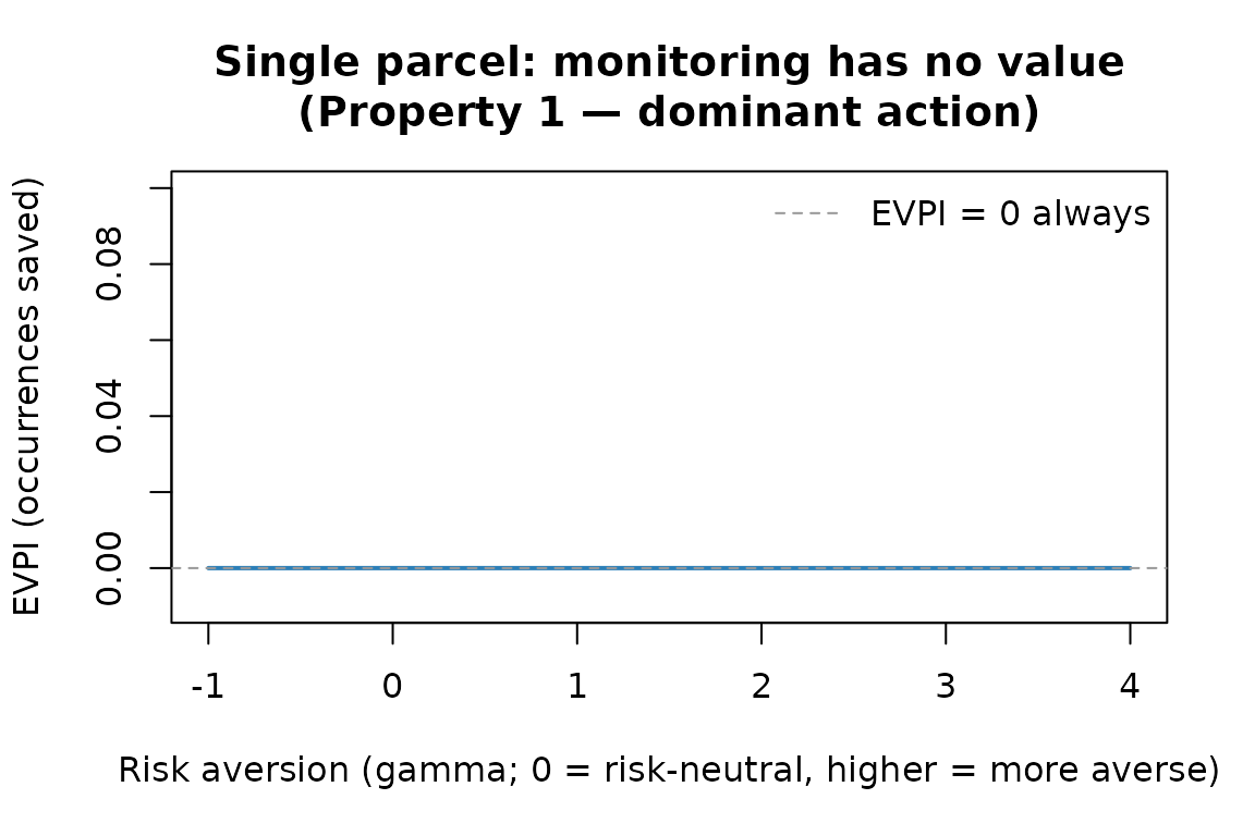

EVPI = 0 for all risk preferences when a dominant action exists (Property 1). Monitoring a single parcel before acting is never worthwhile.

Part 2 — Imperfect monitoring (EVSI) still yields zero

Even with an imperfect survey — say, detection probability of 80 % — the result is the same. Bayes’ theorem updates the probability of presence after each outcome, but “protect” remains optimal in both cases.

detection <- 0.8
p0 <- 0.5  # prior P(present)

# Probability of each survey outcome
p_detected <- p0 * detection
p_not_det  <- 1 - p_detected

# Posterior probability of presence after each outcome (Bayes' theorem)
p_pres_given_det    <- p0 * detection / p_detected
p_pres_given_notdet <- p0 * (1 - detection) / p_not_det

cat("Survey outcome probabilities:\n")
#> Survey outcome probabilities:
cat("  P(detected):              ", round(p_detected, 3), "\n")
#>   P(detected):               0.4
cat("  P(not detected):          ", round(p_not_det,  3), "\n")
#>   P(not detected):           0.6
cat("\nPosterior P(present) after each outcome:\n")
#> 
#> Posterior P(present) after each outcome:
cat("  P(present | detected):    ", round(p_pres_given_det,    3),
    "  -> still protect\n")
#>   P(present | detected):     1   -> still protect
cat("  P(present | not detected):", round(p_pres_given_notdet, 3),
    "  -> still protect\n")
#>   P(present | not detected): 0.167   -> still protect

Because “protect” is optimal after both survey outcomes, the survey cannot change what the manager does — and therefore provides zero value.

p_outcome <- c(detected = p_detected, not_detected = p_not_det)
p_post <- matrix(
  c(p_pres_given_det,    1 - p_pres_given_det,
    p_pres_given_notdet, 1 - p_pres_given_notdet),
  nrow = 2, byrow = TRUE
)

result_evsi <- voi_problem(V_parcel, p_high, p_post, p_outcome) |>
  transform_to_utility() |>
  optimize_action() |>
  calculate_utility_dist() |>
  summarize_utility() |>
  transform_to_values() |>
  calculate_value_info()

cat("EVSI (single parcel, P = 0.5, detection = 0.8):", result_evsi$value_info, "\n")
#> EVSI (single parcel, P = 0.5, detection = 0.8): 0

This is the core result from Bennett et al. (2018): “The best decision for a single parcel only is to ‘protect’ with or without monitoring.”

Part 3 — The budget flip: monitoring becomes valuable

Why the single-parcel result does not generalise

When the manager has many parcels but can only protect some of them, the situation changes fundamentally. The budget forces a prioritisation decision: which parcels get protection and which do not? The dominant-action structure collapses:

A parcel left unprotected loses all benefit, even if the species is there.
Monitoring can reveal which parcels to prioritise.
The effective choice is no longer “protect vs. skip this parcel” but “protect this parcel vs. protect a different parcel instead.”

This is the transition from Property 1 (per-parcel dominant action) to Property 2 (portfolio-level forced trade-off).

Multi-parcel numbers from Bennett et al. (2018)

For a 20-parcel scenario with 10 high-prior parcels (P = 0.5) and 10 low-prior parcels (P = 0.1), and a budget to protect 8 parcels at $5,000 each:

Strategy	Expected occurrences saved
No monitoring: protect the 8 highest-prior parcels	0.5 × 8 = 4.0
Perfect information: protect any 8 parcels known to have the species	6.0
EVPI (portfolio)	2.0 occurrences

The net benefit of monitoring depends on survey costs. Bennett et al. (2018) show that spending $500/parcel × 20 parcels = $10,000 on surveys (equivalent to losing 2 protection slots) still yields a net gain of +1 occurrence — monitoring is worthwhile until survey costs exceed roughly $1,000/parcel.

Two-parcel illustration in vira

The full 20-parcel scenario requires integer programming beyond vira’s scope, but a two-parcel version captures the key structure. With two parcels (high-prior and low-prior) and a budget to protect only one, the decision table covers four states of the world:

p_joint  <- bennett2018_parcel$p_joint
V_budget <- bennett2018_parcel$V_budget

problem_budget <- voi_problem(V_budget, p_joint)

result_budget_rn <- problem_budget |>
  transform_to_utility() |>
  optimize_action() |>
  calculate_utility_dist() |>
  summarize_utility() |>
  transform_to_values() |>
  calculate_value_info()

cat("Two-parcel, budget = protect 1:\n")
#> Two-parcel, budget = protect 1:
cat("  EV without info (protect high-prior parcel):", round(result_budget_rn$EV_uncertainty, 3), "\n")
#>   EV without info (protect high-prior parcel): 0.5
cat("  EV with perfect information:               ", round(result_budget_rn$EV_certainty,   3), "\n")
#>   EV with perfect information:                0.55
cat("  EVPI:                                      ", round(result_budget_rn$value_info,      3), "\n")
#>   EVPI:                                       0.05

With a binding budget, EVPI > 0 even though “protect” dominates at the individual parcel level. The budget removes the effective safe fallback and converts the problem into a Property 2 structure.

Part 4 — Multi-species triage (Case Study 2)

Background

Bennett et al. (2018) present a second case study in which a management agency must decide whether to manage or not manage a group of 20 species whose true threat status is uncertain. The threat classification system is only 50 % accurate, leading to:

True status	Count	Management value if managed
Truly endangered	5 (25 %)	2
Truly threatened	10 (50 %)	1
Truly not threatened	5 (25 %)	0

Not managing yields value 0 regardless of true status. The structure looks similar to the single-parcel case: “manage” seems to weakly dominate. The catch is that monitoring carries a cost: a 0.1 probability per truly endangered species of losing an endangered individual during the monitoring delay.

Summary of results

Scenario	EV result	Property
Single species (manage vs. not)	EVPI = 0	Property 1 (manage dominates)
20-species, budget, imperfect classification	EVSI = +1.2 (RN)	Property 2 at population scale
Same, risk-averse manager	Net benefit < +1.2	RA increases penalty of extinction risk

Single-species decision (EVPI = 0)

Prior: P(endangered) = 0.25, P(threatened) = 0.50, P(not threatened) = 0.25.

“Manage” is strictly better for endangered and threatened species, and equal for not-threatened species. This is a dominant action — a Property 1 structure.

data("bennett2018_multispecies")
V_species <- bennett2018_multispecies$V_species
p_species <- bennett2018_multispecies$p_species

problem_sp <- voi_problem(V_species, p_species)

result_sp_rn <- problem_sp |>
  transform_to_utility() |>
  optimize_action() |>
  calculate_utility_dist() |>
  summarize_utility() |>
  transform_to_values() |>
  calculate_value_info()

cat("EV(manage):          ", sum(V_species[1, ] * p_species), "\n")
#> EV(manage):           1
cat("EV(do not manage):   ", sum(V_species[2, ] * p_species), "\n")
#> EV(do not manage):    0
cat("EV without info:     ", result_sp_rn$EV_uncertainty, "\n")
#> EV without info:      1
cat("EV with perfect info:", result_sp_rn$EV_certainty,   "\n")
#> EV with perfect info: 1
cat("EVPI:                ", result_sp_rn$value_info,       "\n")
#> EVPI:                 0

Published expected value = 0.25 × 2 + 0.5 × 1 + 0.25 × 0 = 1.0 ✓

EVPI = 0: “manage” weakly dominates in all states. Information cannot change what the manager should do for an individual species.

Risk-averse EVPI is also zero

rp_sp <- risk_preference("CRRA", param = 1, val_min = 0, val_max = 2,
                          outcome_name = "management value", maximize = TRUE)
fns_sp <- use_risk_preference(rp_sp)

result_sp_ra <- problem_sp |>
  transform_to_utility(fns_sp$utility) |>
  optimize_action() |>
  calculate_utility_dist() |>
  summarize_utility() |>
  transform_to_values(fns_sp$inv_utility) |>
  calculate_value_info()

cat("EVPI (risk-neutral):", result_sp_rn$value_info,           "\n")
#> EVPI (risk-neutral): 0
cat("EVPI (risk-averse): ", round(result_sp_ra$value_info, 6), "\n")
#> EVPI (risk-averse):  0

As with the single-parcel case, EVPI = 0 under all risk preferences when a dominant safe action exists. No degree of risk aversion can make monitoring valuable when “manage” is always the right call anyway.

How prior uncertainty affects the certainty equivalent

Although the single-species EVPI is always zero, examining how the certainty equivalent changes with the prior gives intuition about where information would become valuable if the action structure changed — for instance, if management had a cost or a budget limited how many species could be managed.

priors_E <- seq(0.01, 0.99, by = 0.01)

ce_no_info <- numeric(length(priors_E))
ce_info    <- numeric(length(priors_E))

for (i in seq_along(priors_E)) {
  pE <- priors_E[i]
  pT <- (1 - pE) / 2
  pN <- (1 - pE) / 2
  p_i <- c(pE, pT, pN)

  res_i <- voi_problem(V_species, p_i) |>
    transform_to_utility(fns_sp$utility) |>
    optimize_action() |>
    calculate_utility_dist() |>
    summarize_utility() |>
    transform_to_values(fns_sp$inv_utility) |>
    calculate_value_info()

  ce_no_info[i] <- res_i$EV_uncertainty
  ce_info[i]    <- res_i$EV_certainty
}

plot(priors_E, ce_no_info, type = "l", lwd = 2, col = "#2c7fb8",
     xlab = "Prior P(truly endangered)",
     ylab = "Certainty equivalent (management value)",
     main = "Single species: CE with and without perfect information",
     ylim = range(c(ce_no_info, ce_info)))
lines(priors_E, ce_info, lwd = 2, col = "#e34a33", lty = 2)
legend("bottomright",
       legend = c("Without information", "With perfect information"),
       col = c("#2c7fb8", "#e34a33"), lty = c(1, 2), lwd = 2, bty = "n")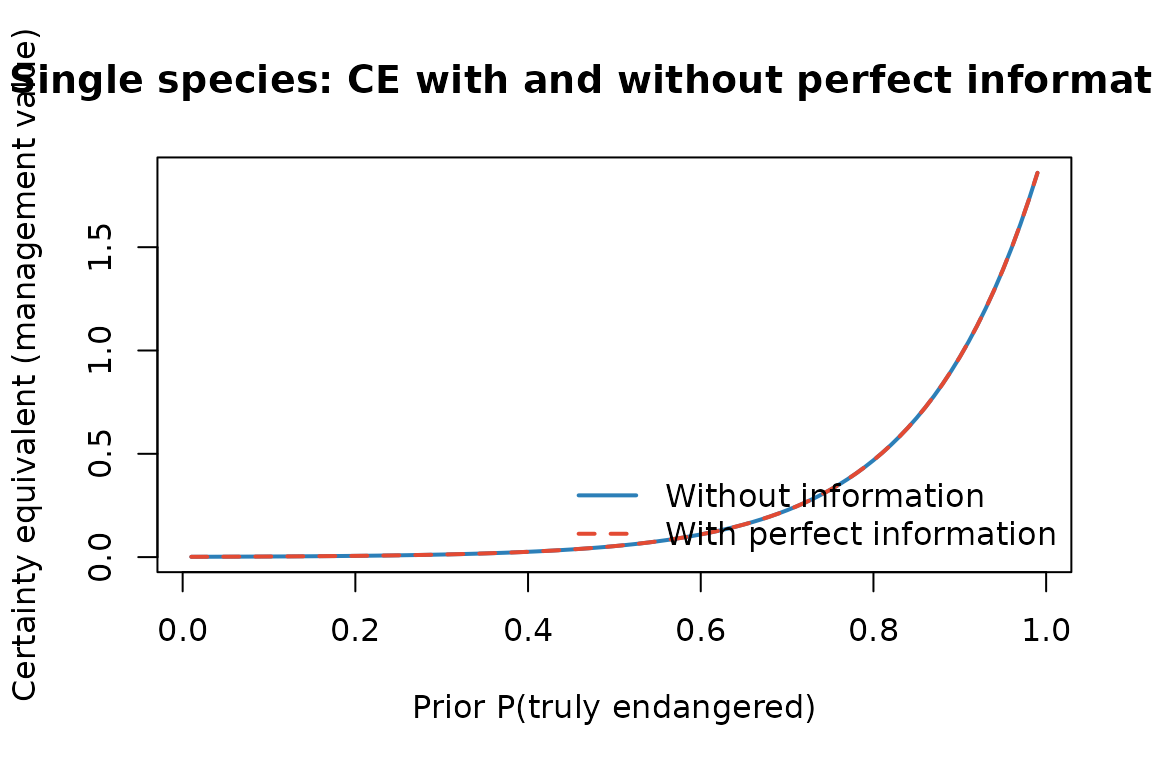

Certainty equivalent with and without perfect information as the prior probability of endangered status varies. The two curves coincide because ‘manage’ is always optimal — confirming EVPI = 0 for all priors.

The two curves coincide throughout — confirming EVPI = 0 for all priors.

Why monitoring is worthwhile at the population scale

Bennett et al. (2018) report that for 20 species with the priors above, the value of monitoring information is +1.2 expected management outcomes (18.2 vs 17.0). Three features drive this reversal from the single-species result:

1. Classification error: the observed threat status is wrong half the time. Monitoring before acting can correct misclassifications and redirect effort to species that actually need it most.

2. No free safe action at scale: a budget allows managing only 17 of the 20 species. The 3 species that go unmanaged lose their management benefit. The choice of which 3 to skip is now a genuine trade-off — and information about true status makes that choice better.

3. Extinction risk during monitoring: each truly endangered species faces a 0.1 probability of extinction during the monitoring delay. For 5 expected endangered species this means 0.5 expected extinctions — a direct cost of monitoring.

Despite this extinction risk, monitoring is worthwhile because correctly re-classifying species allows the agency to target the highest-return units.

Reconstructing the Bennett et al. calculation

n_species <- 20
p_E <- 0.25; p_T <- 0.50; p_N <- 0.25

n_E <- n_species * p_E  # 5 truly endangered
n_T <- n_species * p_T  # 10 truly threatened

v_E <- 2; v_T <- 1

# Without monitoring: all 20 classified as "threatened", manage best 17 (EV = 1 each)
ev_uncertainty <- 1 * 17
cat("EV under uncertainty (manage best 17):          ", ev_uncertainty, "\n")
#> EV under uncertainty (manage best 17):           17

# With perfect information: manage all 5 endangered + all 10 threatened (= 15, within budget)
ev_perfect_info <- n_E * v_E + n_T * v_T
cat("EV with perfect information (manage E + T):     ", ev_perfect_info, "\n")
#> EV with perfect information (manage E + T):      20
cat("EVPI:                                           ", ev_perfect_info - ev_uncertainty, "\n")
#> EVPI:                                            3

# Extinction cost of monitoring delay
n_lost  <- n_E * 0.1      # 0.5 expected extinctions
ev_lost <- n_lost * v_E   # value lost = 0.5 * 2 = 1
cat("\nExpected extinctions during monitoring delay:   ", n_lost, "\n")
#> 
#> Expected extinctions during monitoring delay:    0.5
cat("Value lost to extinction:                       ", ev_lost, "\n")
#> Value lost to extinction:                        1

# With monitoring (imperfect, 50% accurate): from Bennett et al. 2018, Table 7
ev_with_mon <- 18.2
cat("\nEV with monitoring (Table 7):                   ", ev_with_mon, "\n")
#> 
#> EV with monitoring (Table 7):                    18.2
cat("Net value of monitoring (EVSI):                 ", ev_with_mon - ev_uncertainty, "\n")
#> Net value of monitoring (EVSI):                  1.2

Published net monitoring value = 18.2 − 17.0 = +1.2 (Bennett et al. 2018, Table 7). This reflects imperfect monitoring (50 % classification accuracy) combined with the 0.5 expected extinctions during monitoring. The gain from correcting misclassifications outweighs the loss, so monitoring is justified under risk-neutral preferences.

Risk aversion: when the extinction cost dominates

Under risk aversion, the extinction risk during monitoring looms larger than the expected-value calculation suggests. Losing an endangered species (value 2) when it could have been protected carries extra disutility for a risk-averse manager.

To quantify this, we model the monitoring decision explicitly as a choice between:

Act now: manage immediately, no extinction risk, but without the information gain.
Monitor first: gather information to target management better, but accept the 0.025 probability of an endangered individual being lost during monitoring.

p_mon <- bennett2018_multispecies$p_mon
V_mon <- bennett2018_multispecies$V_mon

problem_mon <- voi_problem(V_mon, p_mon)

# Risk-neutral: compare acting now vs monitoring first
result_mon_rn <- problem_mon |>
  transform_to_utility() |>
  optimize_action() |>
  calculate_utility_dist() |>
  summarize_utility() |>
  transform_to_values() |>
  calculate_value_info()

# Risk-averse: same comparison, with penalty on the extinction outcome
rp_mon  <- risk_preference("CRRA", param = 1, val_min = 0, val_max = 2,
                            outcome_name = "species value", maximize = TRUE)
fns_mon <- use_risk_preference(rp_mon)

result_mon_ra <- problem_mon |>
  transform_to_utility(fns_mon$utility) |>
  optimize_action() |>
  calculate_utility_dist() |>
  summarize_utility() |>
  transform_to_values(fns_mon$inv_utility) |>
  calculate_value_info()

cat("EV(act now):                    ", sum(V_mon[1, ] * p_mon), "\n")
#> EV(act now):                     1
cat("EV(monitor first):              ", sum(V_mon[2, ] * p_mon), "\n")
#> EV(monitor first):               0.95
cat("Net benefit of monitoring (RN): ", round(result_mon_rn$value_info, 4), "\n")
#> Net benefit of monitoring (RN):  0
cat("Net benefit of monitoring (RA): ", round(result_mon_ra$value_info, 4),
    "(gamma = 1)\n")
#> Net benefit of monitoring (RA):  0 (gamma = 1)

sens_mon <- voi_sensitivity(problem_mon, rp_mon,
                             param_grid = seq(-1, 4, by = 0.1))

plot(sens_mon$param, sens_mon$voi,
     type = "l", lwd = 2, col = "#7fcdbb",
     xlab = "Risk aversion (gamma; 0 = risk-neutral, higher = more averse)",
     ylab = "Net benefit of monitoring (species value units)",
     main = "Multi-species monitoring: benefit falls with risk aversion")
abline(h = 0, lty = 2, col = "grey50")
legend("topright",
       legend = c("Net monitoring benefit", "Break-even (benefit = 0)"),
       lty = c(1, 2), col = c("#7fcdbb", "grey50"), lwd = c(2, 1), bty = "n")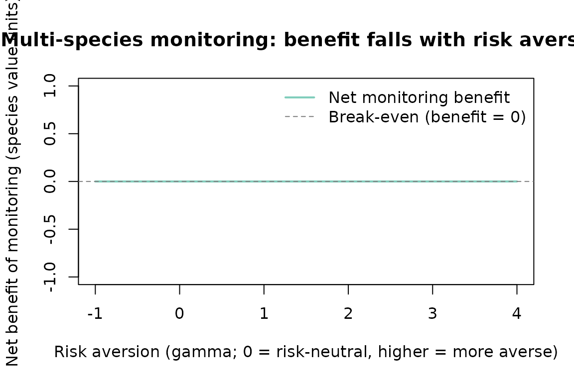

Net benefit of monitoring falls as risk aversion increases. A strongly risk-averse manager may prefer to act immediately, because the small probability of extinction during monitoring is penalised heavily.

A strongly risk-averse manager may prefer to act immediately despite the monitoring information loss, because the irreversible extinction risk carries extreme disutility. The crossover point — where risk aversion tips the decision toward acting without monitoring — depends on the specific extinction probability, the value of endangered species, and the information gain from the survey.

Summary

Scenario	EVPI (risk-neutral)	Property
Single parcel, P = 0.5	0	Property 1 — protect dominates
Single parcel, P = 0.1	0	Property 1 — protect dominates
Single parcel, EVSI (detection = 0.8)	0	Property 1 — protect still dominates
Two parcels, budget = protect 1	> 0	Budget converts to Property 2
Single species (manage vs. not)	0	Property 1 — manage dominates
20 species, budget, imperfect classification	+1.2 (EVSI)	Property 2 at population scale

The budget constraint is the key. Without it, “protect/manage” is always the right answer and monitoring is never worth the effort. With it, the manager faces a genuine prioritisation decision — and information about which units actually need action becomes valuable.

References

Bennett, J.R., Maxwell, S.L., Martin, A.E., Chadès, I., Fahrig, L. & Gilbert, B. (2018). When to monitor and when to act: Value of information theory for multiple management units and limited budgets. Journal of Applied Ecology, 55, 2102–2113. DOI: 10.1111/1365-2664.13132

Property 1 per unit; budget and multi-species scale force Property 2

Key terms used in this vignette

What this vignette shows

Part 1 — Single parcel: protecting always wins

Background

Decision table

EVPI is zero for any prior

EVPI is also zero under risk aversion

Part 2 — Imperfect monitoring (EVSI) still yields zero

Part 3 — The budget flip: monitoring becomes valuable

Why the single-parcel result does not generalise

Multi-parcel numbers from Bennett et al. (2018)

Two-parcel illustration in vira

Part 4 — Multi-species triage (Case Study 2)

Background

Summary of results

Single-species decision (EVPI = 0)

Risk-averse EVPI is also zero

How prior uncertainty affects the certainty equivalent

Why monitoring is worthwhile at the population scale

Reconstructing the Bennett et al. calculation

Risk aversion: when the extinction cost dominates

Summary

References