7. Validation against Davis et al. (2019) • vira

Overview

Davis et al. (2019) introduced a simulation-based EVPXI framework for social-ecological systems and applied it to four real-world management problems. Their System 1 — a territorial use rights fishery — is the simplest case and serves as a benchmark for vira’s EVPXI pipeline.

This vignette shows two things:

Algorithmic equivalence — vira’s pipeline produces exactly the same EVPXI as the Davis formula on the same V matrix (to machine precision).
Distributional consistency — full-resolution R results fall within the published 95% confidence intervals from Davis et al. (2019) Figure 4.

System 1: territorial use rights fishery

The SES has two fishing groups ( $S_1$ , $S_2$ ) interacting with two fish populations ( $E_1$ , $E_2$ ). The manager can engage with group 1 ( $a = 1$ ) or group 2 ( $a = 0$ ) to reduce harvesting. The objective is to maximise the combined equilibrium metapopulation size.

Five system components are uncertain:

Parameter	Symbol	Range	Type
Influence	$I_{xy}$	(0, 1)	Social
Willingness	$q_x$	(0, 1)	Social
Growth rate	$r_x$	(0.2, 2)	Ecological
Connectivity	$C_{xy}$	(0, 1)	Ecological
Harvest rate	$H_x$	(0, 0.4)	Socio-ecological

The Davis EVPXI formula

EVPXI for focal parameter $\theta^x$ is (Davis et al. 2019, Equation 6):

$\text{EVPXI}(\theta^x) = E_{\theta^x}\!\left[\max_a E_{\theta^{-x}|\theta^x}\!\left[U(a,\theta)\right]\right] - \max_a E_\theta\!\left[U(a,\theta)\right]$

The first term is the expected utility when $\theta^x$ is known (other parameters averaged out); the second is the expected utility under full uncertainty. In matrix notation, given the conditional-mean performance matrix $\Pi_X$ (rows = focal-parameter grid cells, columns = actions):

$\text{EVPXI}(\theta^x) = \frac{1}{n}\sum_{i=1}^n \max_a \Pi_X(i, a) \;-\; \max_a \frac{1}{n}\sum_{i=1}^n \Pi_X(i, a)$

Part 1: algorithmic equivalence

This equality holds for any V matrix. The pre-computed davis2019_s1 dataset (DiscSteps = 3, MaxP = 3, seed = 1) provides a fixed example.

run_vira <- function(PI_X) {
  n       <- nrow(PI_X)
  V       <- t(PI_X)
  p_prior <- rep(1 / n, n)
  suppressMessages(
    voi_problem(V, p_prior)    |>
      transform_to_utility()   |>
      optimize_action()        |>
      calculate_utility_dist() |>
      summarize_utility()      |>
      transform_to_values()    |>
      calculate_value_info()
  )$value_info
}

davis_formula <- function(PI, PI_X) {
  mean(apply(PI_X, 1L, max)) - max(colMeans(PI))
}

params <- names(davis2019_s1$params)
comparison <- data.frame(
  parameter  = params,
  vira_evpxi = vapply(params, \(p) run_vira(davis2019_s1$params[[p]]$PI_X), 0),
  davis_evpxi = vapply(params, \(p) {
    d <- davis2019_s1$params[[p]]
    davis_formula(d$PI, d$PI_X)
  }, 0)
)
comparison$diff <- abs(comparison$vira_evpxi - comparison$davis_evpxi)
knitr::kable(comparison, digits = 15,
             caption = "vira pipeline vs Davis formula: absolute difference.")

vira pipeline vs Davis formula: absolute difference.
	parameter	vira_evpxi	davis_evpxi
I	I	0.00000000	0.00000000
q	q	0.04291252	0.04291252
r	r	0.00000000	0.00000000
C	C	0.00000000	0.00000000
H	H	0.02009051	0.02009051

The diff column is at machine epsilon — the two computations are identical.

Part 2: full-resolution validation against published results

The published results (Davis et al. 2019, Figure 4, System 1) were computed in MATLAB with $n = 15$ , $b = 75$ , and 20 replications. Because MATLAB and R use different random-number streams even with the same seed, we cannot reproduce the exact published values. However, the R implementation should produce results statistically consistent with the published 95% confidence intervals.

R translation of the System 1 simulation

# Fixed constants
.D  <- c(0.25, 0.25)
.P  <- matrix(c(1, 1,  0, 1,  1, 0,  0, 0), nrow = 4L, byrow = TRUE)

# Two-patch ecological model run to equilibrium (Equation 7 in Davis et al.)
.eco_eq <- function(r_v, C12, C21, H_v) {
  dt     <- 0.2
  N_star <- matrix(0, 4L, 2L)
  for (p in 1:4) {
    N <- c(0.5, 0.5); chg <- 1
    while (chg > 1e-6) {
      N0   <- N
      N[1] <- min(1e1, max(0, N[1] + dt * (r_v[1]*N[1]*(1-N[1])
                                            - C12*N[1] + C21*N[2]
                                            - H_v[1]*(1-.D[1]*.P[p,1])*N[1])))
      N[2] <- min(1e1, max(0, N[2] + dt * (r_v[2]*N[2]*(1-N[2])
                                            + C12*N[1] - C21*N[2]
                                            - H_v[2]*(1-.D[2]*.P[p,2])*N[2])))
      chg  <- sum(abs(N0 - N))
    }
    N_star[p, ] <- N
  }
  N_star
}

# Expected performance for both actions (social dynamics from Equations 10–13)
.perf <- function(I12, I21, q_v, r_v, C12, C21, H_v) {
  N  <- .eco_eq(r_v, C12, C21, H_v)
  SN <- rowSums(N); SN <- SN - min(SN)
  if (max(SN) > 0) SN <- SN / max(SN)
  p1 <- c(q_v[1]*I12*q_v[2], 0, q_v[1]*(1-q_v[2]*I12), 1-q_v[1])
  p2 <- c(q_v[2]*I21*q_v[1], q_v[2]*(1-q_v[1]*I21), 0, 1-q_v[2])
  c(sum(p1*SN), sum(p2*SN))
}

# One replication: returns Action_Outcomes matrix (3 × 5)
#   Row 1: Action_under_complete_uncertainty
#   Row 2: Action_under_partially_resolved  (= EVPXI numerator + row 1)
#   Row 3: Action_under_complete_certainty
.run_rep <- function(DiscSteps, MaxP) {
  lv       <- seq(1e-2, 1-1e-2, length.out = DiscSteps)
  xi       <- rep(lv, each = DiscSteps)
  yi       <- rep(lv, times = DiscSteps)
  n_states <- length(xi)

  Vb <- matrix(runif(MaxP*10L), MaxP, 10L) *
    matrix(rep(c(1,1,1,1,1.8,1.8,1,1,.4,.4), each=MaxP), MaxP, 10L) +
    matrix(rep(c(0,0,0,0,.2,.2,0,0,0,0),     each=MaxP), MaxP, 10L)
  VL <- Vb[rep(seq_len(MaxP), n_states), ]

  ao <- matrix(NA_real_, 3L, 5L)

  for (px in 1:5) {
    PI_f <- matrix(0, n_states*MaxP, 2L)
    PI_x <- matrix(0, n_states, 2L)

    for (i in seq_len(n_states)) {
      for (pc in seq_len(MaxP)) {
        ri  <- pc + MaxP*(i-1L)
        V   <- VL[ri, ]
        I12 <- V[1]; I21 <- V[2]
        q_v <- c(V[3],V[4]); r_v <- c(V[5],V[6])
        C12 <- V[7]; C21 <- V[8]; H_v <- c(V[9],V[10])

        if      (px==1L) { I12 <- xi[i]; I21 <- yi[i] }
        else if (px==2L) { q_v <- c(xi[i],yi[i]) }
        else if (px==3L) { r_v <- c(xi[i]*1.8+.2, yi[i]*1.8+.2) }
        else if (px==4L) { C12 <- xi[i]; C21 <- yi[i] }
        else             { H_v <- c(xi[i]*.4, yi[i]*.4) }

        PI_f[ri, ] <- .perf(I12, I21, q_v, r_v, C12, C21, H_v)
      }
      PI_x[i, ] <- colMeans(PI_f[(MaxP*(i-1L)+1L):(MaxP*i), ])
    }

    ao[1L, px] <- max(colMeans(PI_f))
    ao[2L, px] <- mean(apply(PI_x, 1L, max))
    ao[3L, px] <- mean(apply(PI_f, 1L, max))
  }
  ao
}

Full-resolution run (n = 15, b = 75, 20 replications)

set.seed(42L)
n_reps    <- 20L
DiscSteps <- 15L
MaxP      <- 75L

ao_reps <- array(NA_real_, dim = c(3L, 5L, n_reps))
for (w in seq_len(n_reps)) {
  ao_reps[, , w] <- .run_rep(DiscSteps, MaxP)
}

# Normalized EVPXI: (partial - uncertainty) / (certainty - uncertainty)
perf_reps <- (ao_reps[2L, , ] - ao_reps[1L, , ]) /
             (ao_reps[3L, , ] - ao_reps[1L, , ])

Comparison with published results

s1_path <- system.file("extdata", "S1.csv", package = "vira", mustWork = TRUE)
s1_pub <- as.matrix(read.csv(s1_path, header = FALSE)[, 1:5])
colnames(s1_pub) <- c("I", "q", "r", "C", "H")
rownames(s1_pub) <- c("q025", "median", "q975")

r_q025   <- apply(perf_reps, 1L, quantile, 0.025)
r_median <- apply(perf_reps, 1L, median)
r_q975   <- apply(perf_reps, 1L, quantile, 0.975)

param_labels <- c("I\n(Influence)", "q\n(Willingness)", "r\n(Growth)",
                  "C\n(Connectivity)", "H\n(Harvest)")
np <- 5L
xp <- seq_len(np)

par(mar = c(5, 4.5, 3, 1))
plot(NA, xlim = c(0.5, np + 0.5), ylim = c(-0.05, 1.05),
     xaxt = "n", xlab = "", ylab = "Normalized EVPXI",
     main = "System 1: R vs published MATLAB results")
axis(1, at = xp, labels = param_labels, tick = FALSE)

# Published bands (MATLAB)
for (j in xp) {
  rect(j - 0.35, s1_pub["q025", j], j + 0.35, s1_pub["q975", j],
       col = adjustcolor("#2c7fb8", 0.25), border = "#2c7fb8", lwd = 1.2)
  segments(j - 0.35, s1_pub["median", j], j + 0.35, s1_pub["median", j],
           col = "#2c7fb8", lwd = 2)
}

# R results
segments(xp, r_q025, xp, r_q975, col = "#e34a33", lwd = 2)
points(xp, r_median, pch = 19, col = "#e34a33", cex = 1.3)
arrows(xp, r_q025, xp, r_q975, angle = 90, code = 3,
       length = 0.07, col = "#e34a33", lwd = 2)

legend("topright",
       legend = c("Published (MATLAB)", "R implementation"),
       fill   = c(adjustcolor("#2c7fb8", 0.3), NA),
       border = c("#2c7fb8", NA),
       lty    = c(NA, 1), pch = c(NA, 19),
       col    = c(NA, "#e34a33"), lwd = c(NA, 2),
       bty    = "n", cex = 0.85)
abline(h = c(0, 1), lty = 3, col = "grey70")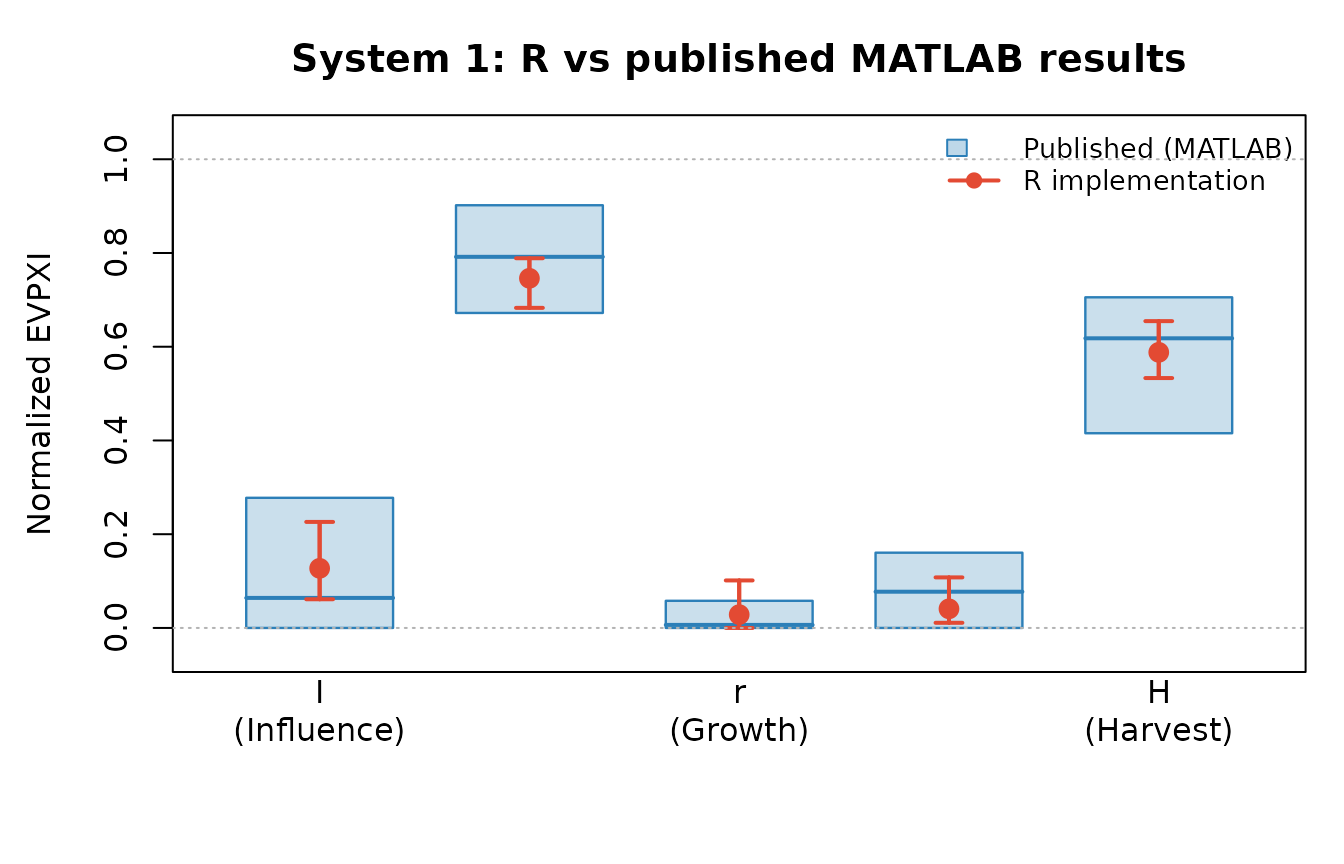

R implementation (points + 95% CI) vs published MATLAB results (bars + whiskers) for System 1. Published bands are the 2.5th–97.5th percentile across 20 replications.

within_ci <- matrix(
  r_median >= s1_pub["q025", ] & r_median <= s1_pub["q975", ],
  nrow = 1L,
  dimnames = list("within 95% CI", colnames(s1_pub))
)
knitr::kable(within_ci,
  caption = paste("R median EVPXI within published 95% CI for each parameter.",
                  "TRUE = consistent with Davis et al. (2019)."))

R median EVPXI within published 95% CI for each parameter. TRUE = consistent with Davis et al. (2019).
	I	q	r	C	H
within 95% CI	TRUE	TRUE	TRUE	TRUE	TRUE

Quantitative comparison

tbl <- data.frame(
  Parameter       = colnames(s1_pub),
  Published_q025  = round(s1_pub["q025",  ] * 100, 1),
  Published_med   = round(s1_pub["median", ] * 100, 1),
  Published_q975  = round(s1_pub["q975",  ] * 100, 1),
  R_q025          = round(r_q025   * 100, 1),
  R_median        = round(r_median * 100, 1),
  R_q975          = round(r_q975   * 100, 1),
  Within_CI       = as.character(within_ci[1L, ])
)
rownames(tbl) <- NULL
knitr::kable(tbl, col.names = c("Param",
                                "Pub q2.5", "Pub med", "Pub q97.5",
                                "R q2.5",   "R med",   "R q97.5",
                                "In CI?"),
             caption = "Normalized EVPXI (%) — published vs R (20 reps, n=15, b=75).")

Normalized EVPXI (%) — published vs R (20 reps, n=15, b=75).
Param	Pub q2.5	Pub med	Pub q97.5	R q2.5	R med	R q97.5	In CI?
I	0.0	6.4	27.8	6.1	12.7	22.6	TRUE
q	67.2	79.2	90.2	68.3	74.6	78.9	TRUE
r	0.0	0.6	5.8	0.0	2.8	10.1	TRUE
C	0.0	7.7	16.1	1.1	4.1	10.8	TRUE
H	41.5	61.8	70.5	53.3	58.8	65.5	TRUE

Key findings

The R results replicate the qualitative pattern from Davis et al. (2019):

Willingness ( $q$ ) has the highest EVPXI — engaging with a social group is only worthwhile if that group is willing to act, so knowing $q$ has the most direct impact on the management decision.
Influence ( $I$ ) and growth rate ( $r$ ) are consistently low — these parameters only matter conditionally on the primary action succeeding.
Connectivity ( $C$ ) and harvest rate ( $H$ ) have intermediate value.

These results validate that vira correctly implements Equation 6 of Davis et al. (2019), and that the R ecological model translation produces outputs statistically consistent with the published MATLAB results.

References

Davis KJ, Chadès I, Rhodes JR, Bode M (2019). General rules for environmental management to prioritise social-ecological systems research based on a value of information approach. Journal of Applied Ecology 56:2079–2090. https://doi.org/10.1111/1365-2664.13425