2. Expected Value of Perfect Information (EVPI)

The chytrid frog problem

We use the translocation problem from Canessa et al. (2015), introduced in vignette 1. The manager chooses to translocate frogs or do nothing; the outcome depends on whether chytrid fungus is present (50 % prior). Full background is in vignette 1.

data("canessa2015")
V <- canessa2015$V
p <- canessa2015$p

Quick start: one-line EVPI

For a risk-neutral calculation, calculate_evpi() handles everything and prints a formatted decision table:

result_rn <- calculate_evpi(V, p, outcome_name = "frogs")
#>       action chytrid_present chytrid_absent EV_prior best_action?
#>  translocate              55            135       95             
#>    no_action             100            100      100          YES

The EVPI of 17.5 frogs matches the published value (Canessa et al. 2015).

Use survey_worth_it() to compare this against a proposed survey cost:

survey_worth_it(result_rn, survey_cost = 10)
survey_worth_it(result_rn, survey_cost = 20)

---

Step-by-step pipe (for full control)

The one-liner above runs six steps internally. Here they are individually, with a plain-English description of each.

problem <- voi_problem(V, p)

Step 1 — transform_to_utility() Converts outcomes (frog counts) into “preference units”. In the risk-neutral case nothing changes — every frog counts equally. Under risk aversion this step bends the scale so that avoiding bad outcomes carries extra weight.

Step 2 — optimize_action() Finds the best action in two situations: (a) acting now with our current beliefs, and (b) acting after the survey for each possible result. This determines when and how the survey changes the decision.

Step 3 — calculate_utility_dist() Evaluates the outcome of the chosen action across all possible states of the world, producing a distribution of results.

Step 4 — summarize_utility() Collapses that distribution to a single number — by default the expected (average) value.

Step 5 — transform_to_values() Converts the summary back from preference units into the original outcome units (frogs). In the risk-neutral case this is a no-op.

Step 6 — calculate_value_info() Subtracts: value with perfect information minus value without. This difference is the EVPI.

result_rn2 <- problem |>
  transform_to_utility() |>
  optimize_action() |>
  calculate_utility_dist() |>
  summarize_utility() |>
  transform_to_values() |>
  calculate_value_info()

result_rn2$value_info
#> [1] 17.5

View the decision table at any point after optimize_action():

problem |>
  transform_to_utility() |>
  optimize_action() |>
  decision_table()
#>       action chytrid_present chytrid_absent EV_prior best_action?
#>  translocate              55            135       95             
#>    no_action             100            100      100          YES

---

Risk-averse EVPI: the certainty equivalent

Under risk aversion, the decision-maker cares not just about the average outcome but about the worst-case risk. We express VOI as the difference in certainty equivalents — the guaranteed frog count the manager would accept in place of the uncertain outcome.

rp  <- risk_preference("CRRA", param = 1, val_min = 0, val_max = 200,
                        outcome_name = "frogs", maximize = TRUE)

result_ra <- calculate_evpi(V, p, rp = rp, outcome_name = "frogs")
#>       action chytrid_present chytrid_absent EV_prior best_action?
#>  translocate              55            135       95             
#>    no_action             100            100      100          YES

The certainty equivalent EVPI is lower than the risk-neutral EVPI. Under risk aversion, the best action under uncertainty (no translocation) already provides a safe floor of 100 frogs regardless of state — which a risk-averse manager values highly. Perfect information therefore adds less on top.

cat("CE under certainty:  ", round(result_ra$EV_certainty, 2), "frogs\n")
#> CE under certainty:   116.19 frogs
cat("CE under uncertainty:", round(result_ra$EV_uncertainty, 2), "frogs\n")
#> CE under uncertainty: 100 frogs
cat("EVPI (CE):           ", round(result_ra$value_info, 2), "frogs\n")
#> EVPI (CE):            16.19 frogs

How EVPI varies with risk aversion

sens <- voi_sensitivity(problem, rp, param_grid = seq(-0.5, 4, by = 0.1))

plot(sens$param, sens$voi,
     type = "l", lwd = 2, col = "#2c7fb8",
     xlab = "Risk aversion (gamma)", ylab = "EVPI (frogs)",
     main = "Sensitivity of EVPI to risk aversion")
abline(v = rp$param, lty = 2, col = "grey40")
legend("topright", legend = "gamma = 1 (log utility)",
       lty = 2, col = "grey40", bty = "n")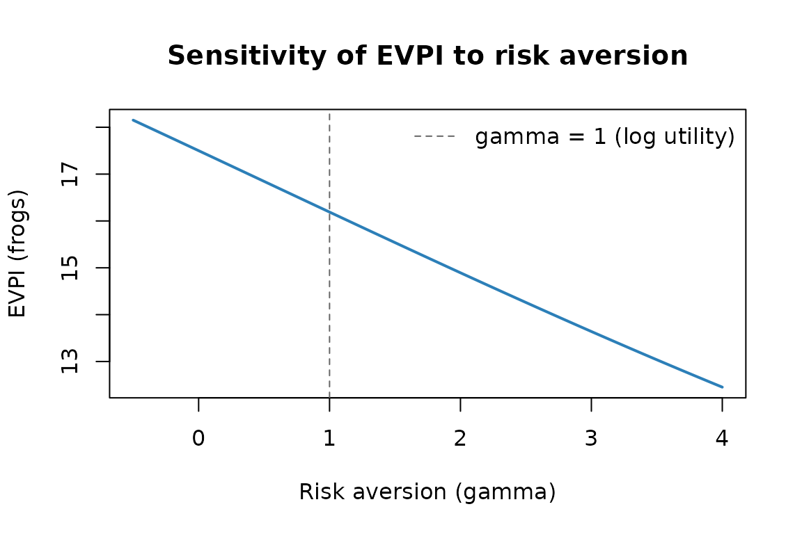

EVPI (certainty equivalent) decreases as risk aversion increases.

At gamma = 0 (risk-neutral) EVPI = 17.5. As risk aversion increases, the safe no-translocation action becomes increasingly preferred regardless of state, reducing the value of resolving uncertainty.